
Multiband HF Center‑Loaded Off‑Center‑Fed Dipoles
Serge Stroobandt, ON4AA
Copyright 2007–2021, licensed under Creative Commons BY-NC-SA
- Home
- Antenna Designs
- CL-OCFDs

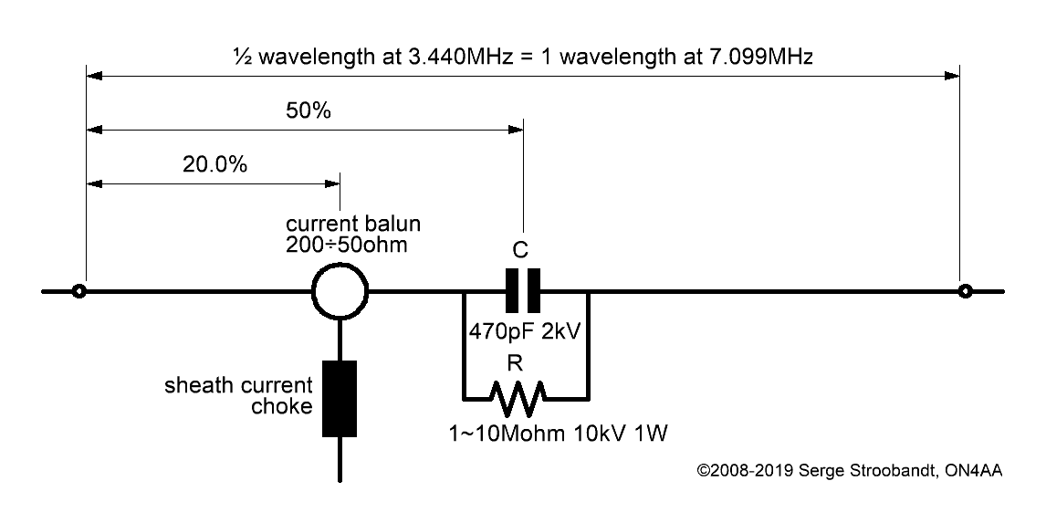
ON4AA’s CL-OCFD with 80, 40, 30, 20, 15 & 10 m coverage. The capacitor C shortens the dipole for 80 m (actually 75 m) band resonance, whereas the coil lengthens the dipole for 30 m third harmonic resonance. Resistor R has as sole function bleeding off static charges, protecting capacitor C.
ON4AA’s 80, 40, 20, 15, 12 & 10m CL-OCFD. The capacitor C renders the dipole resonant on the 80 (actually 75) meter band, while resistor R has as sole function bleeding off static charges, hence protecting capacitor C. There is no third harmonic resonance on 30 m. However, in return, seventh harmonice resonance is present on 12 m.
Having any questions about the CL-OCFD antenna?
Wanting to discuss OCFDs and single-wire-fed Windom antennas?
Post your questions, results and pictures to:
the OCFD

Design goals
 output tank of a PA
- Like many fellow radio amateurs, I own a fairly standard shortwave radio station consisting of a 100 W HF transceiver driving a 1 kW tube power amplifier. I never chose to spend any money on a kW-rated antenna-tuner. Anyhow, I can tune out VSWRs as high as 3÷1 with the adjustable pi-network of the output filter tank inside my power amplifier.
Thus I set out to design an HF antenna with a VSWR of 3÷1, or less, over the full bandwidth of as many amateur radio HF bands as possible. At the same time, my preference went out to the low- and the non-WARC bands. This design exercise resulted in a new kind of antenna which I dubbed Center-Loaded Off-Center-Fed Dipole Antenna, or CL-OCFD for short.
The Center-Loaded Off-Center-Fed Dipole (CL-OCFD) was invented and first described by yours truly, Serge Y. Stroobandt, ON4AA, in the year 2006. I briefly considered patenting my design. However, I chose not to do so as a way to give back to this wonderful hobby community, which indirectly has given me a lot. If you like or use the CL-OCFD, please, consider making a donation towards keeping this site on‑line.
Companies or individuals selling any CL-OCFD antenna variant are granted the explicit permission to do so, but are kindly solicited to refer the inventor by name and call sign in any manual and marketing material.
Performance
 on target
- In proof of its performance, an EZNEC-calculated VSWR-graph of the CL-OCFD antenna is presented in Figure 2. This antenna works without a tuner over the entire bandwidth of the 80, 40, 30, 20, 15 and 10 m-band, simply by adjusting the output-tank of your tube power amplifier. —If your final output stage is a transistor amplifier, you definitely will need an antenna-tuner though.— In such, this antenna is the first described single-wire antenna to be offering these capabilities.
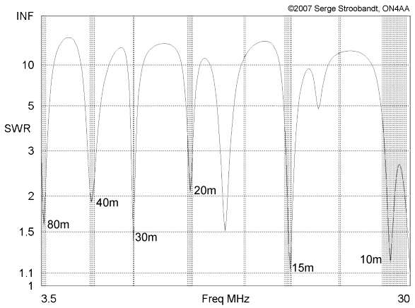
VSWR of the 80, 40, 30, 20, 15 & 10m CL-OCFD as a function of frequency
Why off-center-fed?
When offsetting the feed position of a dipole antenna away from its center, at some point, similar feed impedances can be obtained for a number of frequency bands. This occurs at the fundamental (λ/2 dipole) resonant frequency as well as a number of harmonic resonant frequencies.
This is possible because a standing wave is present along the dipole which causes the feed impedance to change. In the span of a quarter wavelength, it varies from a very high value at the antenna ends (several kΩ) to the value of the radiation resistance at the corresponding frequency.
At its fundamental resonant frequency, in free space and for an infinitesimal thin wire, the dipole’s theoretical center feed impedance would be 73 Ω. However, the optimal multiband feed point will have a higher impedance than this theoretical center feed impedance. Hence, a good quality impedance-transforming balun will be necessary to match the optimal balanced feed impedance to that of the unbalanced coaxial feed cable.
Full 80 m-band coverage
 full 80 m-band coverage
- Operating a center-fed dipole over the entire 80 m-band turns out to be particularly challenging. With 8.2% relative bandwidth the 80 m-band (3.5–3.8 MHz) is exceptionally broad. Cumbersome cage dipoles or load switching arrangements deliver only partially satisfactory results.
However, any OCF dipole easily outperforms aforementioned obtrusive antenna arrangements.1,2 Here is why:
Placing the feed point away from the center, increases the resistive part of the feed impedance and source load more than the reactive (imaginary) part of the resonant antenna, which is nearly resonant. This effectively lowers the loaded Q-factor of the antenna at the feed point. Offsetting the feed position of a dipole antenna, will result in a lower loaded Q-factor and hence a broader working bandwidth at the fundamental frequency.
\[{Q_\text{loaded}\downarrow}\equiv\frac{X_\text{in}}{R_\text{in}\uparrow+R_\text{source}\uparrow}\quad\textrm{and}\quad Q_\text{loaded}=\frac{f_\text{res}}{BW}\quad\Rightarrow\quad{BW\uparrow}\,=\frac{f_\text{res}}{Q_\text{loaded}\downarrow}\]
In summary, offset feeding causes the antenna to be loaded differently. The effect is most pronounced at the fundamental frequency. This is a first reason why it pays off to build your OCF dipole with 80 m as the fundamental wavelength and not, for example, 160 m. An additional reason will be given in the section about center-loading.
Please note that a year after the publication of this article, Eugene G. Preston, K5GP, described a dualband 160 & 80 m CL-OCFD exhibiting comparable broadband behaviour on 80 meter.3 However, this 80 m broadband performance is achieved in a slightly different manner. The antenna is actually a 3-band CL-OCFD antenna (160, 80 & 75 m) where the center loading moves the natural third harmonic to the lower end of the 80 m band, below the 75 m second harmonic.
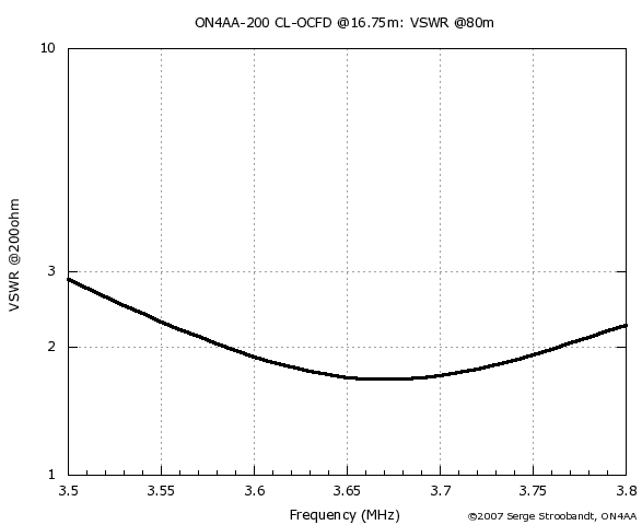
VSWR of the six-band CL-OCFD on 80 m and at a height of 16.75 m (55 ft)
Literature
 continuous renewal
- Rather than reinventing the wheel, every antenna project should start with a quick literature study of similar published antenna designs. Doing so for the multiband Windom or off-center-fed dipole antenna (see table below), leads to a stunning revelation. Over many years, antenna dimensions and feed locations have not changed much from the original single-wire design, whereas balun feed impedances have decreased from 500 Ω to 300 or even 200 Ω! This, of course, is reason enough to become very suspicious about published multiband Windom designs.
| design | year | Zin | ℓtot | ℓshort | offset* | hagl | config. | bands |
|---|---|---|---|---|---|---|---|---|
| W8GZ | 1929 | 500 Ω | 0.483 λ | 0.18 λ | 37.3% | single wire fed | single band | |
| VS1AA4 | 1937 | 500 Ω | 41.00 m | 13.60 m | 33.2% | single wire fed | 80† 40 20 17 12 10 m | |
| K4ABT | 1949 | 200 Ω | 40.5 m | 13.4 m | 33.1% | 6–12 m | horiz. | 80 40 20 17 12 10 m |
| DJ2KY5 | 1971 | 300 Ω | 42 m | 14 m | 33.3% | horiz. | ||
| “FD4”4 | 1971 | 300 Ω | 41.45 m | 13.50 m | 32.6% | 8 m | inv.-V | 80† 40 20 17 12 10 m |
| “FD4”6 | 1971 | 300Ω | NA‡ | NA‡ | NA‡ | top: 12 m ends: 8 & 3 m |
asymm. inv.-V | 80† 40 20 17 12 10 m |
| K8SYH | 70’s | 300 Ω | 39.08 m | 12.74 m | 32.6% | horiz. | ||
| I7SWX7,8 | 1988 | 300 Ω | 41.0 m | 13.5 m | 32.9% | horiz. | ||
| JA7KPI | 1994 | 200 Ω | 41.0 m | 13.6 m | 33.2% | 11 m | inv.-V | 80 40 20 17 10 m |
| K3MT | 1997 | 450 Ω | 42.06 m | 12.65 m | 30.1% | top: 14 m ends: 5 m | asymm. inv.-V | 80† 40 20 17 15 12 10 m |
| ON4BAA | 2002 | 300 Ω | 41.00 m§ | 8.10 m | 19.8% | 14 m | horiz. | 80† 40 20 15 12 10 m |
| ON4BAA | 2003 | 200 Ω | 41.00 m§ | 6.25 m | 15.2% | 14 m | horiz. | 80 40 20 17 10 m |
| W8JI | 2006 | 300 Ω | 41.8 m | 8.35 m | 20.0% | horiz. | 80† 40 20 15 10 m | |
| ON4AA | 2007 | 200 Ω | 40.66 m§ | 11.76 m | 28.9% | 17 m | horiz. center-load |
80 40 30 20 15 10 m |
| K5GP | 2008 | 200 Ω | 74.67 m | 14 m | 18.75% | 5.5 m | horiz. | 160 80 75 m |
| ON4AA | 2018 | 200 Ω | 40.66 m§ | 8.13 m | 20.0% | 15 m | horiz. center-load |
80 40 20 15 12 10 m |
| ON4AA | 2018 | 200 Ω | 40.66 m§ | 8.13 or 11.76 m | 20.0% or 29.3% | 15 m | horiz. center-load |
80 40 30 20 15 10 m |
Table notes:
- * The open end of the antenna corresponds to 0% offset, the middle of the dipole to 50%.
- † VSWR ≤ 3÷1 only within a narrow portion of the 80 m-band.
- ‡ Inconsistent data in brochure; end-insulator separation and heights do not correspond to angle between dipole legs at specified height.
- § Antenna made of soft PVC insulated HO7 V-K 4 wire.
As a matter of fact, I first made this table in 2002, when I held the call ON4BAA. It promptly triggered me to start using the power of computer modelling to study this poorly understood antenna. This resulted in two designs; a 300 Ω and a 200 Ω design. Both had feeding locations much closer to the antenna end than usual. This improved the VWSR-performance quite a bit. In 2006, Tom Rauch, W8JI, reproduced these findings with a slightly longer bare copper wire antenna.
However, two problems remained:
- Although the traditional OCF dipole had very broad band-segments, the VSWR-minima of either the 80 m or the 40 m-band could not be perfectly aligned to the respective band-centers. Also, designs that did better on 80 m, lack 15 m. Apparently, OCF dipole designs had so far been a compromise between these three bands. The renowned “FD4” antenna was not an exception; Have a look at its VSWR specification on pages 13 and 14 of this brochure.
- Furthermore, none of these designs offered 30 m. This is a pity, because most hams would put up a wire antenna especially for the lower bands where beam antennas are more difficult to erect.
The next section explains why traditional OCF dipoles have these inherent limitations. Rest assured, both problems are dealt with by the CL-OCFD, also listed at the bottom of Table 1.
Resonant lengths
- It is often said that the HF amateur radio bands are harmonics of the 80 m-band. But is this really the case? The statement can easily be tested by considering a horizontal wire at a practical height (16.75 m or 55 ft) above a typical city lot (σ = 1 mS/m; εr = 5). I use gauge 4 mm² copper wire insulated by a 0.8 mm-thick layer of soft PVC. For the remainder of only this section, the length of the wire is such that it achieves λ/2 dipole resonance at the geometric center frequency fc of the Region I 80 m-band (3.647 MHz). At the geometric center frequency of every other band, we will now determine how much wire needs to be added or subtracted to achieve harmonic resonance. It should be very little if the bands were truly harmonic.
Note that bare copper wire at higher heights and above better ground would yield longer resonant lengths, due to less capacitive coupling to the ground. Either way, this does not affect the validity of what follows. Let us now look at the even and odd harmonics in separate groups, starting with the even harmonics.
Even harmonics
Table 2 clearly shows that the lower band-edges are exactly harmonic; all frequencies are integer multiples of 7.000 MHz. All even harmonic bands also have similar relative bandwidths; i.e. higher harmonic bands become proportionally wider. (The FM-portion of the 10 m-band is temporarily left out of consideration.) Consequently, the geometric center frequencies of the even harmonic bands are also more or less harmonic and their harmonic resonant lengths almost equal. This is reflected in a low value for the standard deviation of the harmonic resonant lengths. In conclusion, it must be relatively easy to design an off-center-fed dipole for this set of even harmonics, provided we find a feed position with comparable feed impedances for all of these frequencies.
In this example, the arithmetic mean of the even harmonic resonant lengths is 40.66 m (133.4 ft). The mean resonant length corresponds to a fundamental resonant frequency of 3.440 MHz. We will keep this in mind for trimming our antenna once it is hung.
| band | fl (MHz) | fu (MHz) | fc (MHz) | harmonic | length | Δ |
|---|---|---|---|---|---|---|
| 40 m | 7.000 | 7.200 | 7.099 | 2 | 40.52 m | -0.14 m |
| 20 m | 14.000 | 14.350 | 14.174 | 4 | 40.75 m | 0.09 m |
| 15 m | 21.000 | 21.450 | 21.224 | 6 | 40.87 m | 0.22 m |
| 10 m | 28.000 | 29.200 | 28.594 | 8 | 40.49 m | -0.17 m |
| arithmetic mean | 40.66 m | |||||
| standard deviation | 0.16 m |
Odd harmonics
| band | fl (MHz) | fu (MHz) | fc (MHz) | harmonic | length | XCL |
|---|---|---|---|---|---|---|
| 80 m | 3.500 | 3.800 | 3.647 | 1 | 38.68 m | -j91 Ω |
| 30 m | 10.100 | 10.150 | 10.125 | 3 | 42.76 m | +j241 Ω |
| 17 m | 18.068 | 18.168 | 18.118 | 5 | 39.89 m | -j153 Ω |
| 12 m | 24.890 | 24.990 | 24.940 | 7 | 40.61 m | -j12 Ω |
| standard deviation | 1.48 m |
Let us continue and have a look now at the odd harmonics. The situation turns out completely different. Even though 3.500 MHz is exactly one half of 7.000 MHz, the resonant length of the 80 m-band is, at its geometric center frequency, much shorter than the mean resonant length of the even harmonic bands. This is because, with 8.2%, the 80 m band has the broadest relative bandwidth of all amateur HF bands. It easily surpasses the 5.9% of the entire 10 m-band (28.000–29.700 MHz).
The 30 m band is equally problematic, being not even a real harmonic. Its resonant length is much longer than the mean of 40.66 m for the even harmonics.
Finally, we see that 17 and 12 m behave very well. The resonant length of the 12 m-band nearly coincides with the mean resonant length of the even harmonic bands.
Remember the problems with the OCF antennas discussed in the previous literature survey? This should no longer astonish us. Above tables revealed that the resonant lengths of the 80 and 30 m bands are true outliers compared to the harmonic resonant lengths of the other HF bands. It is the underlying cause for the partial 80 m coverage and the complete absence of 30 m-band coverage in prevalent OCF antenna designs.
Read on to see how both problems can be solved.
Center-loading
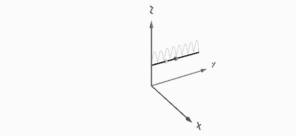
Below diagram shows the current distribution along an antenna wire for its first eight harmonic resonances. The current distributions of the even harmonics are plotted above the wire, those of the odd harmonics below. Do you notice anything special?

Current distribution of the first eight harmonic resonances along an antenna wire
 inspiring book cover
- At least, I do. It may seem trivial, but all even harmonics have (almost) zero current at the center of the antenna, whereas all odd harmonics experience a current maximum at this location.
Zero current for the even harmonics at the center, implies that I can literally do what I want at the center of the antenna without upsetting the even harmonics. I can even cut the antenna in two! As a matter of fact, this is precisely what we are going to do!
It might seem unfortunate that the wavelengths of the 80 m and 30 m-bands are too short, respectively, too long to be true harmonics of the other bands. However, luck struck upon seeing that both problematic bands happen to be odd harmonics. Please, note that this statement does not hold when considering a double-sized OCFD with 160 m as the fundamental frequency. This antenna design is therefore not scalable!
What remains to be done now, is to cut the antenna in half and insert a center-loading network in series. This network will need to add the necessary center loading reactances XCL (see Table 3 above) in order to render the antenna resonant at the odd harmonics. As mentioned before, resonance makes matching at multiple frequencies a lot easier.
Capacitive center load
Let’s start easy. When we have a 40.66 m (133.4 ft) long wire hanging in our garden, at least we would like it to be also perfectly resonant on the popular 80 m-band. Table 3 told us that the wire is too long for resonance at 80 m. A capacitive reactance of -j91.3 Ω needs to be put in series at the center of the antenna. At 3.647 MHz this corresponds to **a center load capacitor of 478 pF, say 470 pF.
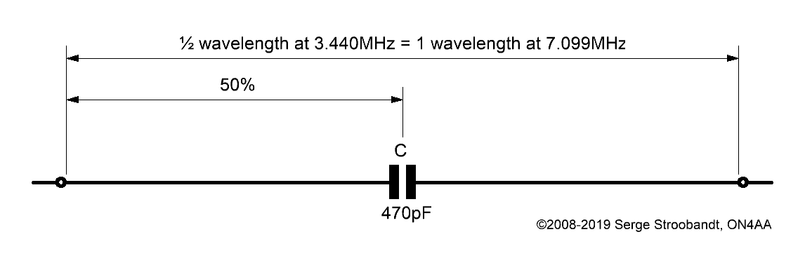
A center-loaded wire, resonant on six bands; four even harmonics (40, 20, 15 & 10 m) and one odd harmonic (80 m). The capacitor has a nominal value of 470 pF. Its effective capacitance should be about 478 pF at 3.647 MHz.
However, by placing this capacitor at the center, we will upset the other odd harmonic resonances, namely 30 and 17 m. By coincidence, the antenna remains resonant on the odd harmonice of 12 m because the capacitor of 470 pF corresponds to a reactance of -j13.5 at 24.990 MHz.
Series LC center load
Now let us try to regain another odd harmonic, in addition to the already recovered 80 m band. For some, but not all odd harmonics, this can be done by loading the center of the antenna with a series LC network (see Table 4).
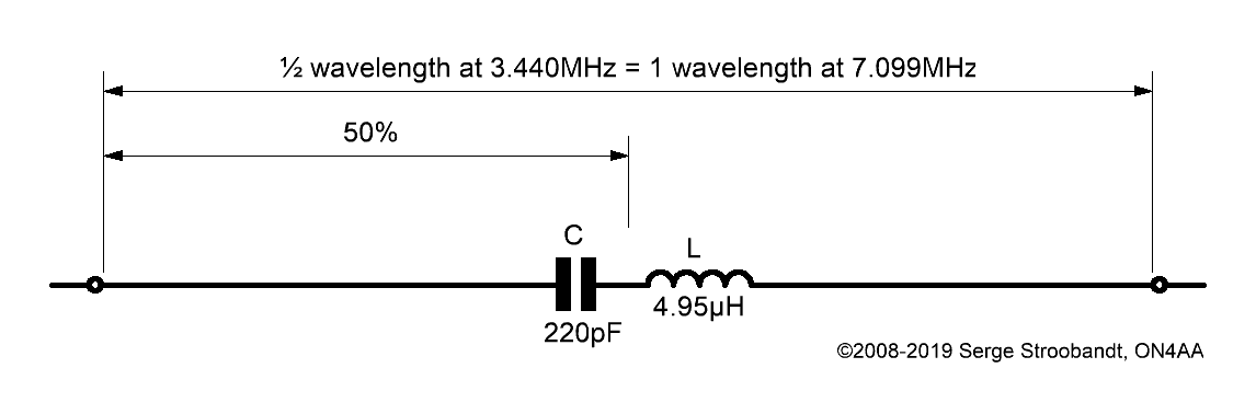
A center-loaded wire, resonant on six bands; four even harmonics (40, 20, 15 & 10 m) and two odd harmonics (80 & 30 m)
| fodd (MHz) | XCL @f | odd harmonics | C | L | fres (MHz) | XL @f |
|---|---|---|---|---|---|---|
| 3.647 | -j91.3 Ω | 80 m | 478 pF | no L | no L | no L |
| 10.125 | +j241 Ω | 80 & 30 m | 213 pF | 4.95 µH | 4.900 | +j314.7 Ω |
| 18.118 | -j153 Ω | 80 & 17 m | 692 pF | no solution! | no solution! | no solution! |
| 24.940 | -j11.8 Ω | 80 & 12 m | 477 pF | 10.1 nH | 72.486 | +j1.58 Ω |
Example: second row in above table
- Placing a 213 pF, say 220 pF, capacitor in series with a 4.95 µH inductor at the center of the antenna will make the antenna resonant at 80 & 30 m, as well as all even harmonics. The resonant frequency of the center load will be 4.900 MHz. At 10.125 MHz, the series inductor L should have a (measured) reactance of +j314.7 Ω. Knowing these values helps with the design and fine-tuning of the series inductor L.
Derivation of series LC center load component values
The center load component values C and L in Table 4, as well as their resonant frequency \(f_\text{res}\) are obtained as follows.
\[\begin{cases}\omega_1L-\frac{1}{\omega_1C}=X_1\quad\text{(I)}\\\omega_2L-\frac{1}{\omega_2C}=X_2\quad\text{(II)}\end{cases}\]
\(\omega_1\) and \(\omega_2\) represent the radial frequencies of the geometric center of any of two odd harmonic bands in Table 4, whereby \(\omega_i=\tau\cdot f_{\text{odd,}i}=2\pi\cdot f_{\text{odd,}i}\), whereas \(X_1\) and \(X_2\) are the required reactances.
\[\text{(I)}\Rightarrow L=\frac{1}{\omega_1}\left[X_1+\frac{1}{\omega_1C}\right]\quad\text{(III)}\]
\[\text{(III) in (II) :}\quad\frac{\omega_2}{\omega_1}\left[X_1+\frac{1}{\omega_1C}\right]-\frac{1}{\omega_2C}=X_2\]
\[\Rightarrow \left[\frac{\omega_2}{\omega_1^2}-\frac{1}{\omega_2}\right]\frac{1}{C}=X_2-\frac{\omega_2}{\omega_1}X_1\]
\[\Rightarrow C=\left[\frac{\omega_2}{\omega_1^2}-\frac{1}{\omega_2}\right]\left[\frac{\omega_1}{\omega_1}X_2-\frac{\omega_2}{\omega_1}X_1\right]^{-1}\]
\[\Rightarrow C=\left[\frac{\omega_2}{\omega_1^2}-\frac{1}{\omega_2}\right]\frac{\omega_1}{\omega_1X_2-\omega_2X_1}=\left[\frac{\omega_2}{\omega_1}-\frac{\omega_1}{\omega_2}\right]\frac{1}{\omega_1X_2-\omega_2X_1}\]
\[\Rightarrow C=\frac{\omega_2^2-\omega_1^2}{\omega_1\omega_2\left(\omega_1X_2-\omega_2X_1\right)}\quad\text{(IV)}\]
Both \(C\) and \(L\) are known at this point, but the expression for \(L\) is further developed:
\[\text{(IV) in (III) :}\quad L=\frac{1}{\omega_1}\left[X_1+\frac{\omega_2\left(\omega_1X_2-\omega_2X_1\right)}{\omega_2^2-\omega_1^2}\right]\]
\[\Rightarrow L=\frac{1}{\omega_1}\left[\frac{\omega_2^2X_1-\omega_1^2X_1+\omega_1\omega_2X_2-\omega_2^2X_1}{\omega_2^2-\omega_1^2}\right]\]
\[\Rightarrow L=\frac{\omega_2X_2-\omega_1X_1}{\omega_2^2-\omega_1^2}\]
Hence, the resonant frequency of the center load:
\[\omega_\text{res}=\frac{1}{\sqrt{LC}}=\left[LC\right]^{-\frac{1}{2}}=\left[\frac{\omega_2X_2-\omega_1X_1}{\omega_1\omega_2\left(\omega_1X_2-\omega_2X_1\right)}\right]^{-\frac{1}{2}}\]
\[\Rightarrow \omega_\text{res}=\sqrt{\omega_1\omega_2\frac{\omega_1X_2-\omega_2X_1}{\omega_2X_2-\omega_1X_1}}\quad\text{and}\quad f_\text{res}=\frac{\omega_\text{res}}{2\pi}\]
More bands?
Yeah, right. Let me disappoint you by saying that things are not as easy as adding just one additional reactive element in series or parallel to obtain yet another band. After all, the center load impedance XCL would have to change sign twice. However, theoretically it should be possible to devise a passive network that makes the antenna resonant on all odd harmonic bands. Nonetheless, such a network will be far from practical to have it hanging along a wire. Moreover, it remains to be seen whether a low VSWR feed point can be found that accommodates all these bands (see next section). The challenge is there for the taker!
As mentioned before, it is not possible to scale this antenna to a longer 160 m-version. Would one try to do so, the problematic 80 m-band would become an even harmonic and hence impossible to be influenced by center-loading the antenna.
The 6 m-band (50–52 MHz) is the 14th harmonic of the 80m-band. Being such a high harmonic, it becomes prohibitively difficult to pinpoint a low VSWR 6 m-band feeding offset.
No resonant traps
Please, do allow me to tackle some anticipated criticism. Uninformed spirits may argue that the two-element network of this antenna is a resonant trap adding significant loss.
This is clearly not the case! The two-element center-loading network is not resonant at any of the amateur bands and is therefore not acting as a trap. It is strictly a loading network, adding relatively little reactance. As such, it does not contribute more loss than any other loading inductors commonly employed in the very best of commercial and home-made low-band Yagi-Uda designs.
Optimal offset & input impedance
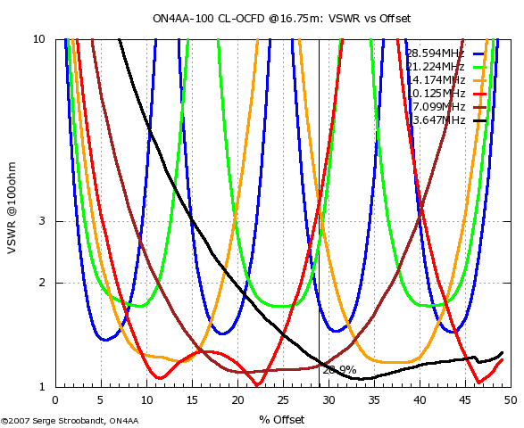
Now that the antenna can be made resonant on six bands, a «sweet spot» needs to be found where VSWR at a given feed impedance is low on all six bands. To determine this ideal feed offset, VSWR graphs at difference feed impedances are plotted for all frequency bands and all possible offset percentages. These are then compared. This is done for the 6-band version of the CL-OCFD which includes 30m resonance. Note that 0% offset corresponds to the open end of the antenna; 50% offset corresponds to the middle of the dipole.
Below graphs were produced with the antenna at 16.75 m (55 ft) over city ground (σ = 1 mS/m; εr = 5) in the near field. Running the model with different ground characteristics revealed that the VSWR of the antenna is barely influenced by the RF properties of the ground underneath (not considering height above the ground for the moment.)
Modelling with 4nec2
Here is the 4nec2 input file of the ON4AA 200 Ω CL-OCFD antenna over good RF ground (σ = 10 mS/m; εr = 14).
The model requires 4nec2 version 5.7.0 or higher.
An EZNEC model is also available.
About rendering VSWR-offset graphs
Here is an interesting fact: every line of every VSWR-offset graph below has been drawn on the basis of 98 data points. Every single of these data point then again resulted from one complete antenna analysis. In other words, six bands times 98 data points, means 588 NEC2 runs were necessary to draw just one complete six-band VSWR-offset graph.
In 2002, the only way to obtain such a graph was by undertaking the monastic task of running EZNEC 98 times and manually copying 1176 numbers —input impedances are complex numbers— onto a spreadsheet. This was done so for every of the four VSWR-offset graphs below.
A couple of years later, this task could be automated, thanks to 4nec2. This excellent antenna modelling interface for NEC2 allows one to sweep any arbitrary antenna variable. What is more, 4nec2 is freeware. Thank you for that, Arie Voors! Nonetheless, as a FLOSS advocate, I am still hoping for Arie to publish the source code. This would safeguard future development should the original developer be no longer around. Even though 4nec2 is coded for MicroSoft Windows™, I run 4nec2 flawlessly on GNU/Linux using the equally free Playon Linux software.
VSWR of the six-band 150 Ω CL-OCFD as a function of feed point offset
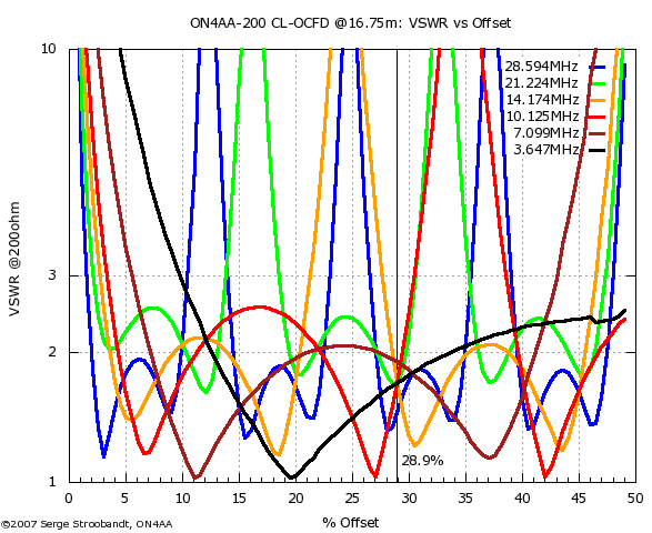
VSWR of the six-band 200 Ω CL-OCFD as a function of feed point offset
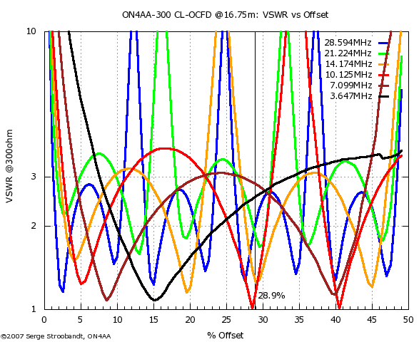
VSWR of the six-band 300 Ω CL-OCFD as a function of feed point offset
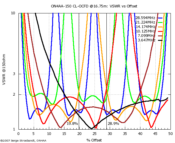
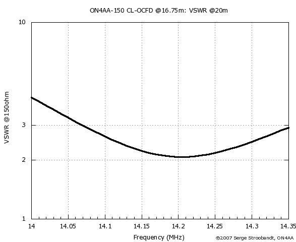
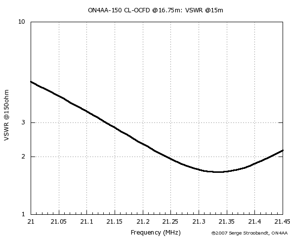
Avoid low-impedance sources
VSWR versus offset plots were rendered for 150 Ω and 100 Ω sources. These plots equally showed points where low VSWR coincided for a number of bands. However, there is one caveat. These VSWR vs. offset plots are for spot frequencies only. At the band edges, VSWR actually increases a lot with low-impedance sources. (Here are examples for 20 m and 15 m with a 150 Ω source at 19.8% offset.) This happens because using a low-impedance source results in an antenna with a higher loaded Q-factor. Only an antenna with a low loaded Q-factor will provide full 80m band coverage, as explained before.
Optimal offset with 200 Ω source
For a feed impedance of 200 Ω, all bands yield a VSWR below 2÷1 at 29.3% offset.
Avoid a 300 Ω source
Feeding the antenna from a 300 Ω source is not desirable since the VSWR will always be high on at least one of the resonant bands.
Avoid high-impedance sources
With high-impedance sources, VSWR minima increasingly coincide at small offsets, eventually resulting in a high-impedance end-fed antenna. However, high-impedance sources come at the price of increased problems with sheath currents, feed point arcing and wide-band transforming losses. These designs do exist, but their analysis is beyond the scope of this article.
Designs
| bands | ℓtot | Zin | offset* | center load |
|---|---|---|---|---|
| 80 40 20 15 12 10 m | λ/2 at 3.440 MHz | 200 Ω | 20.0% | 470 pF† |
| 80 40 30 20 15 10 m | λ/2 at 3.440 MHz | 200 Ω | 20.0% (29.3%) | 220 pF + 4.95 µH |
| 40 20 15 10 m | 3× λ/2 at 21.224 MHz | 200 Ω | 40.5% | — |
Table notes:
- * The open end of the antenna corresponds to 0% offset, the middle of the dipole to 50%.
Only 200 Ω feeds produce practicable results for a true multi-band design. Therefore, a feed impedance of 200 Ω and a feed offset of 20% or 29.3% are kept as the optimal result of this design exercise. Here is how the 200 Ω six-band CL-OCFD will look like when adding a 10 kV 1 W thick film metal oxide resistor R of about 1 to 10 MΩ to bleed off static charges and hence protect the capacitor C from breaking down.
CL-OCFD with 80, 40, 20, 15, 12, & 10 m coverage
The same optimal offset equally applies to the version of the CL-OCFD with 30 m instead of 12 m-band coverage.
CL-OCFD with 80, 40, 30, 20, 15 & 10 m coverage
VSWR
Below VSWR curves were rendered with 4nec2. The six-band CL-OCFD antenna was modelled hanging at 16.75 m (55 ft) above very poor city ground (σ = 1 mS/m; εr = 5). In reality, the VSWR measured in the shack will be lower because of damping by the feed line losses. Here is the 4nec2 input file.
VSWR of the six-band 200 Ω CL-OCFD with 28.9% offset on 80 m
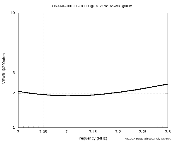
VSWR of the six-band 200 Ω CL-OCFD with 28.9% offset on 40 m
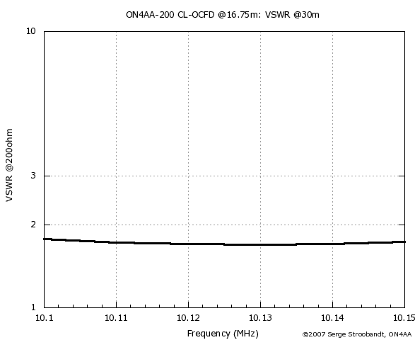
VSWR of the six-band 200 Ω CL-OCFD with 28.9% offset on 30 m
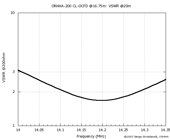
VSWR of the six-band 200 Ω CL-OCFD with 28.9% offset on 20 m
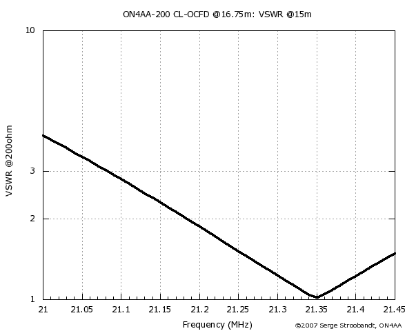
VSWR of the six-band 200 Ω CL-OCFD with 28.9% offset on 15 m
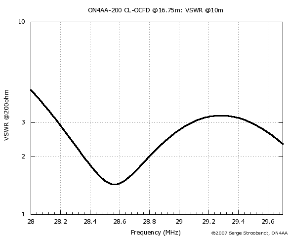
VSWR of the six-band 200 Ω CL-OCFD with 28.9% offset on 10 m
VSWR spectrum sweep
The six-band 200 Ω CL-OCFD with 28.9% offset was also modelled 16.75 m (55 ft) above good RF ground (σ = 10mS/m; εr = 14) using EZNEC.
Modelling with EZNEC
Here is the EZNEC input file. The model employs real ground in the near field of the antenna; not perfect MININEC ground.
A 4nec2 model is also available.
From comparison with previous modelling above very poor city ground, one may conclude that, at least at a height of 16.75 m (55 ft), VSWR is hardly influenced by ground quality. Furthermore, EZNEC in comparison to 4nec2 indicates that the antenna needs to be slightly longer, namely: 40.812 m. Anyhow, a fail-proof trimming procedure will be presented further on.
VSWR of the six-band 200 Ω CL-OCFD as a function of frequency
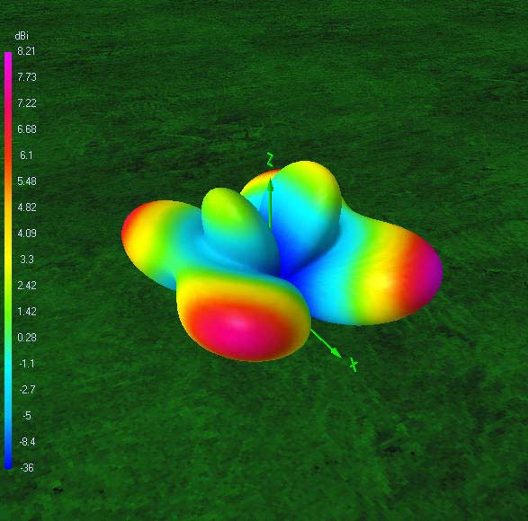
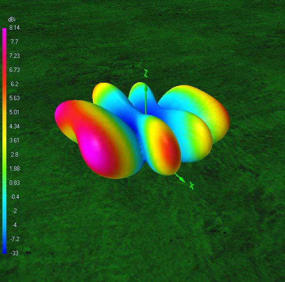
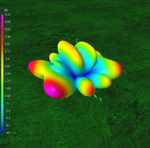
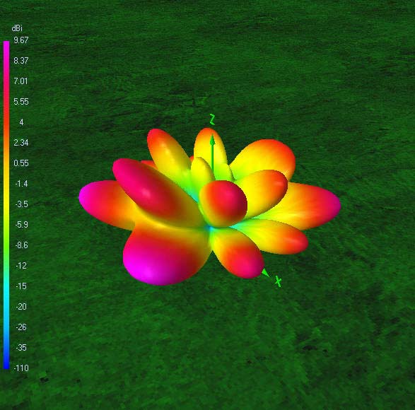
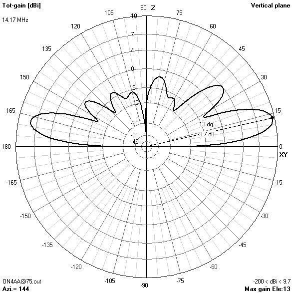
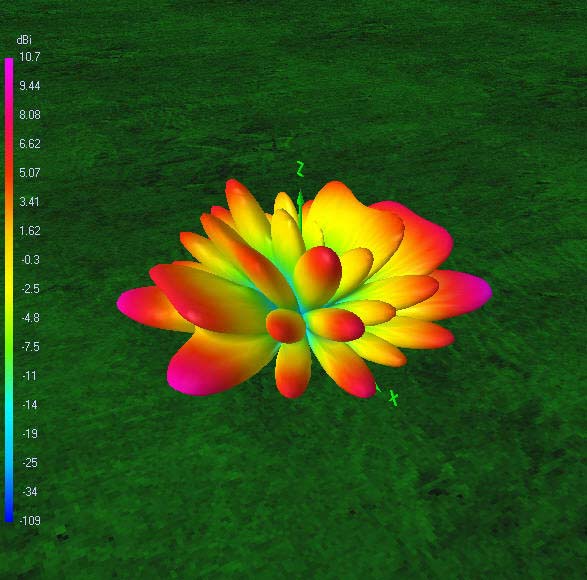
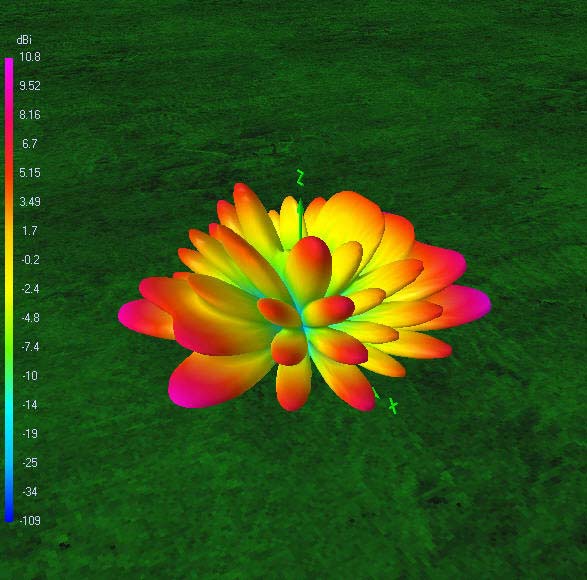
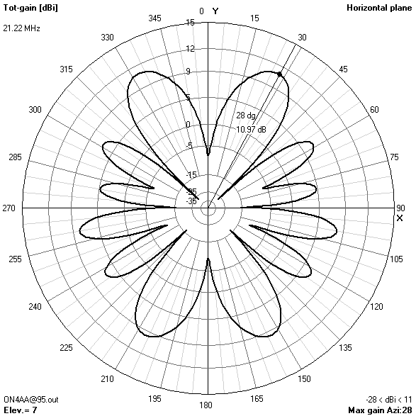
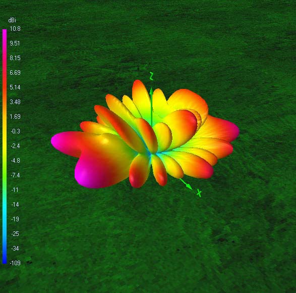
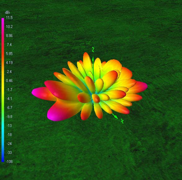
Radiation patterns
The following 72 power gain patterns in dBi were obtained using 4nec2 and good RF ground (σ = 10 mS/m; εr = 14). The 4nec2 input file is available for download.
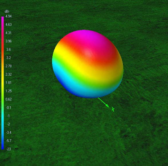
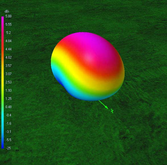
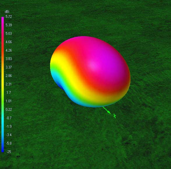
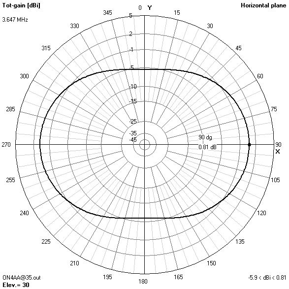
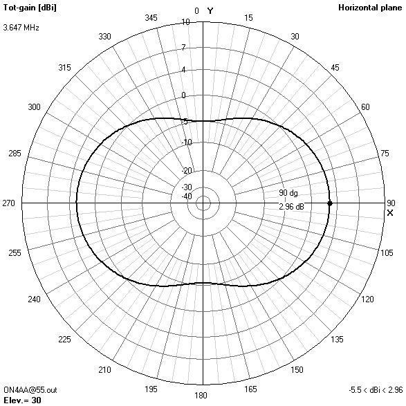
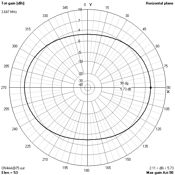
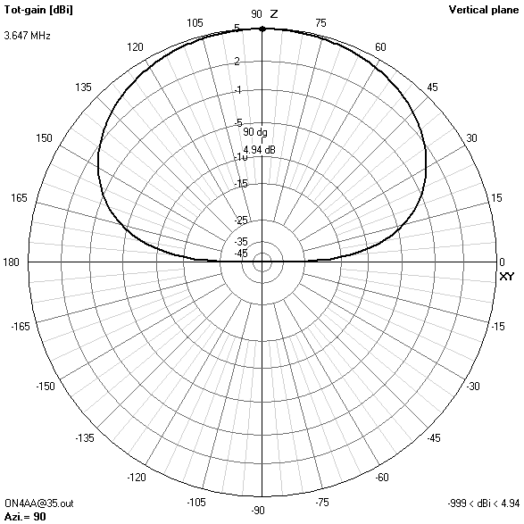
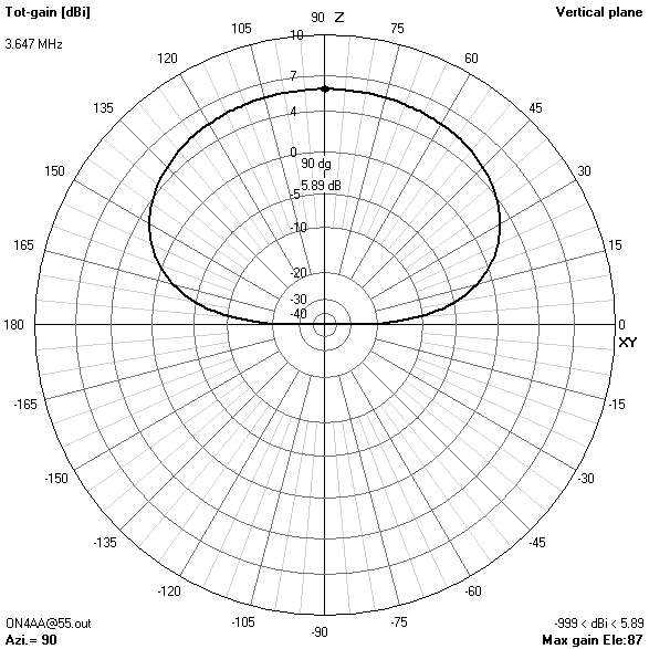
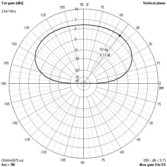
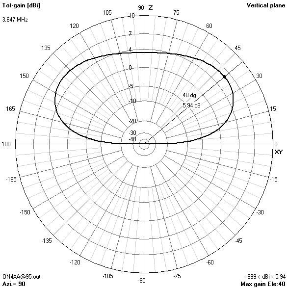
80 m-band radiation patterns
80 m-band or fundamental resonant current distribution
| 10.67 m (35 ft) | 16.76 m (55 ft) | 22.86 m (75 ft) | 28.96 m (95 ft) |
|---|---|---|---|
 \ \ |
 \ \ |
 \ \ |
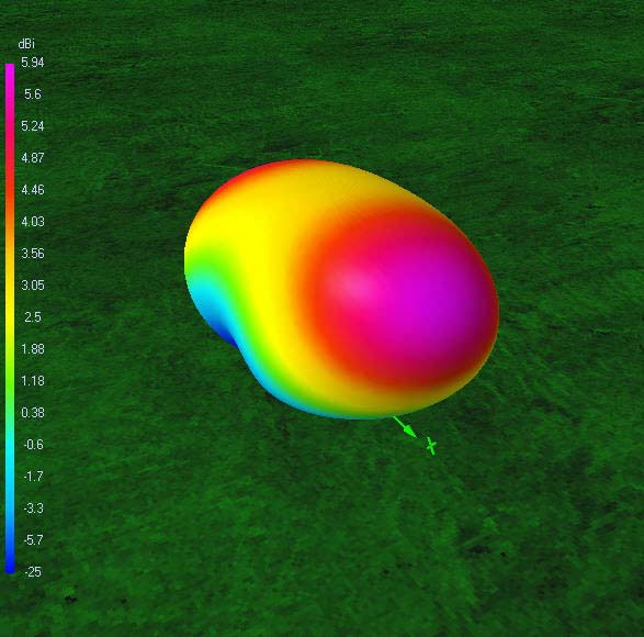 |
| 4.94 dBi ∡ 90° | 5.89 dBi ∡ 90° | 5.73 dBi ∡ 90° | 5.94 dBi ∡ 90° |
 \ \ |
 \ \ |
 \ \ |
 |
 \ \ |
 \ \ |
 \ \ |
 |
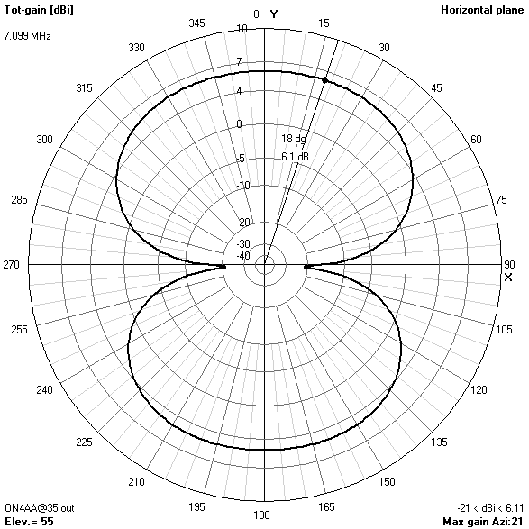
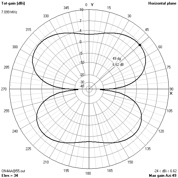
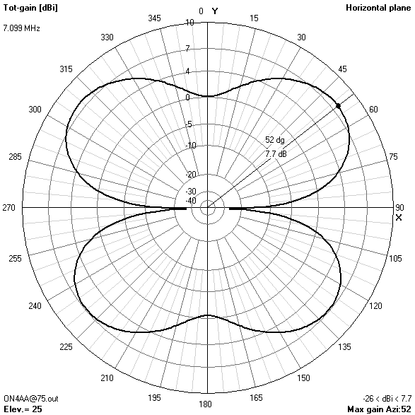
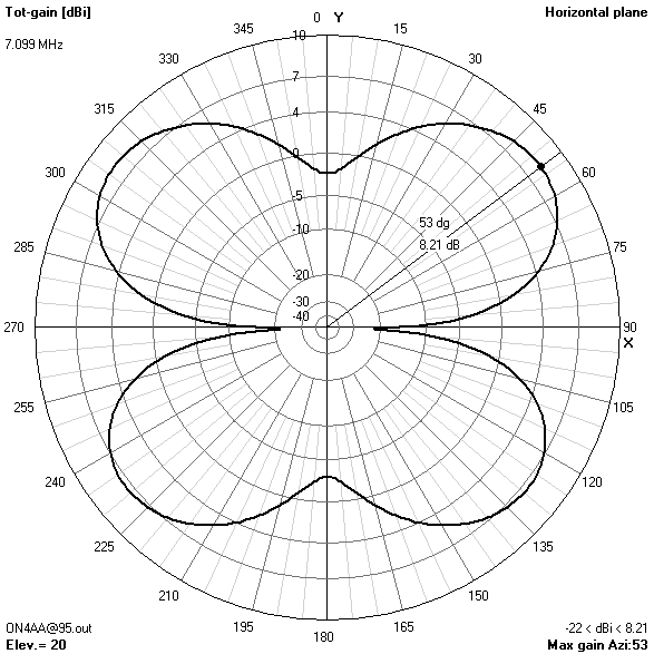
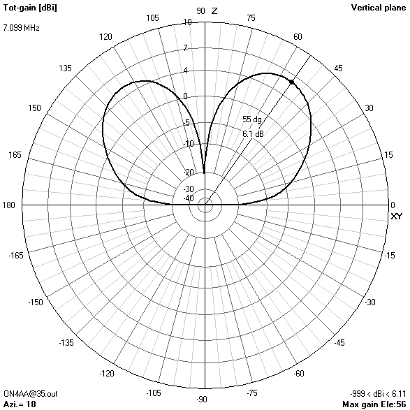
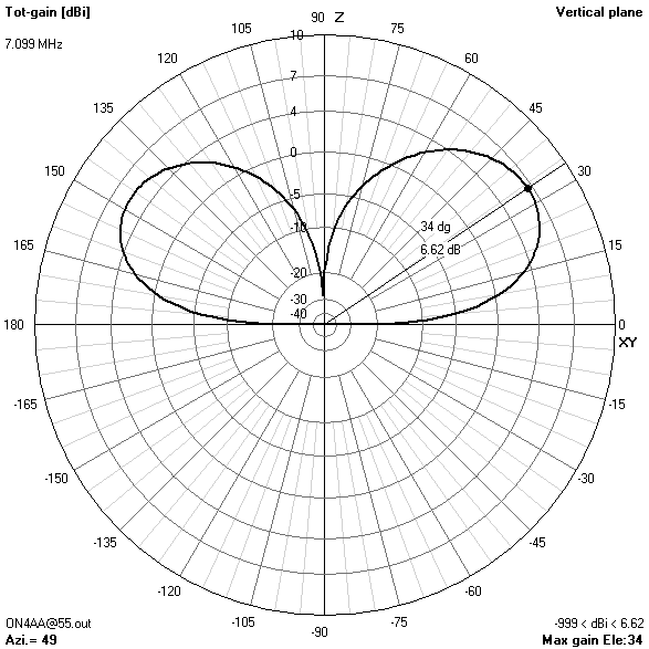
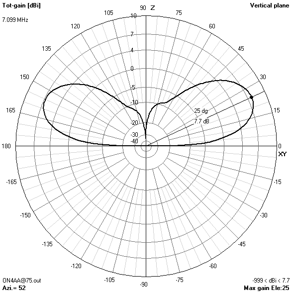
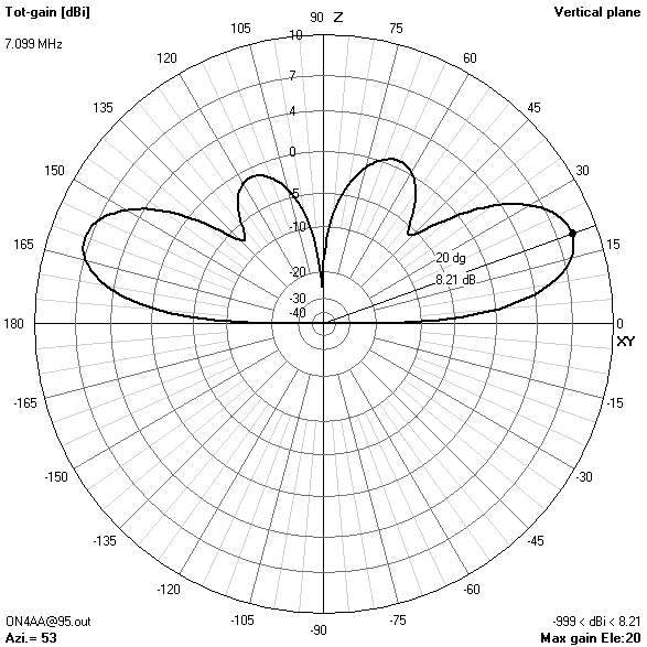
40 m-band radiation patterns

40 m-band or second harmonic current distribution
| 10.67 m (35 ft) | 16.76 m (55 ft) | 22.86 m (75 ft) | 28.96 m (95 ft) |
|---|---|---|---|
 \ \ |
 \ \ |
 \ \ |
 |
| 6.11 dBi ∡ 55° | 6.62 dBi ∡ 34° | 7.70 dBi ∡ 25° | 8.21 dBi ∡ 20° |
 \ \ |
 \ \ |
 \ \ |
 |
 \ \ |
 \ \ |
 \ \ |
 |
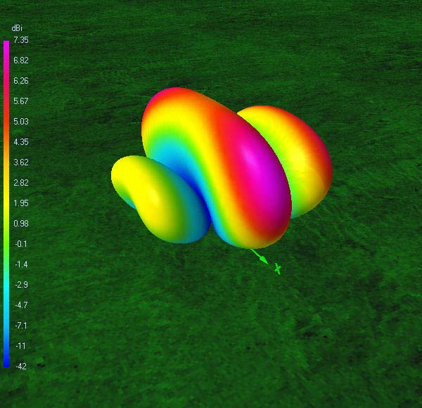
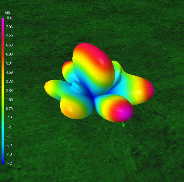
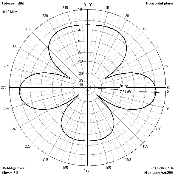
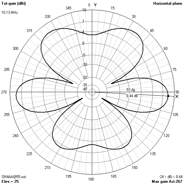
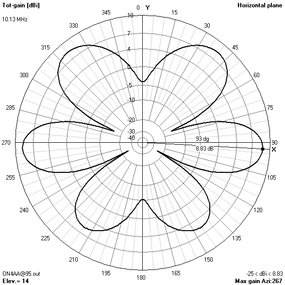
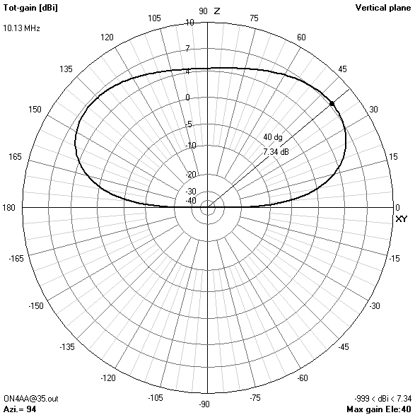
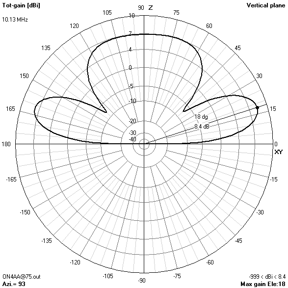
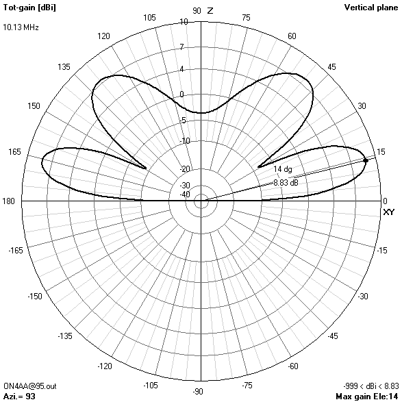
30 m-band radiation patterns

30 m-band or third harmonic current distribution
| 10.67 m (35 ft) | 16.76 m (55 ft) | 22.86 m (75 ft) | 28.96 m (95 ft) |
|---|---|---|---|
 \ \ |
 \ \ |
 \ \ |
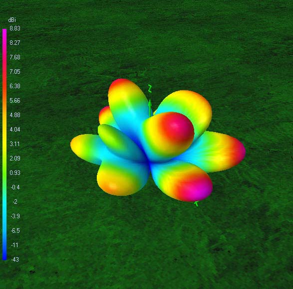 |
| 7.34 dBi ∡ 40° | 8.44 dBi ∡ 25° | 8.40 dBi ∡ 18° | 8.83 dBi ∡ 14° |
 \ \ |
 \ \ |
 \ \ |
 |
 \ \ |
 \ \ |
 \ \ |
 |
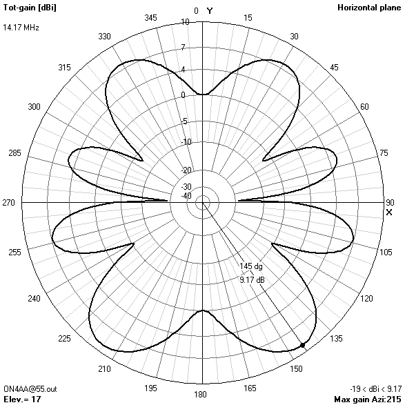
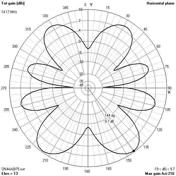
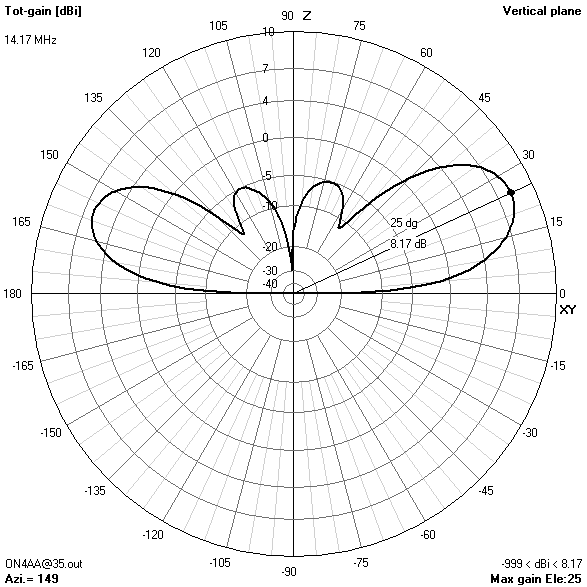
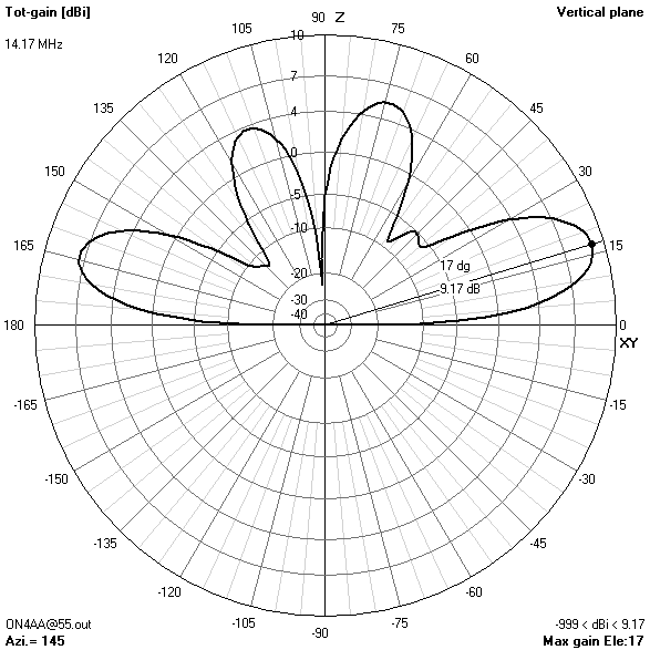
20 m-band radiation patterns

20 m-band or fourth harmonic current distribution
| 10.67 m (35 ft) | 16.7 6m (55 ft) | 22.86 m (75 ft) | 28.96 m (95 ft) |
|---|---|---|---|
 \ \ |
 \ \ |
 \ \ |
 |
| 8.17 dBi ∡ 25° | 9.17 dBi ∡ 17° | 9.70 dBi ∡ 13° | 9.65 dBi ∡ 10° |
 \ \ |
 \ \ |
 \ \ |
 |
 \ \ |
 \ \ |
 \ \ |
 |
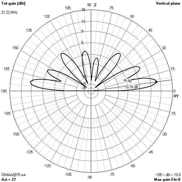
15 m-band radiation patterns

15 m-band or sixth harmonic current distribution
| 10.6 7m (35 ft) | 16.76 m (55 ft) | 22.86 m (75 ft) | 28.96 m (95 ft) |
|---|---|---|---|
 \ \ |
 \ \ |
 \ \ |
 |
| 9.58 dBi ∡ 17° | 10.56 dBi ∡ 11° | 10.78 dBi ∡ 8° | 10.97 dBi ∡ 7° |
 \ \ |
 \ \ |
 \ \ |
 |
 \ \ |
 \ \ |
 \ \ |
 |
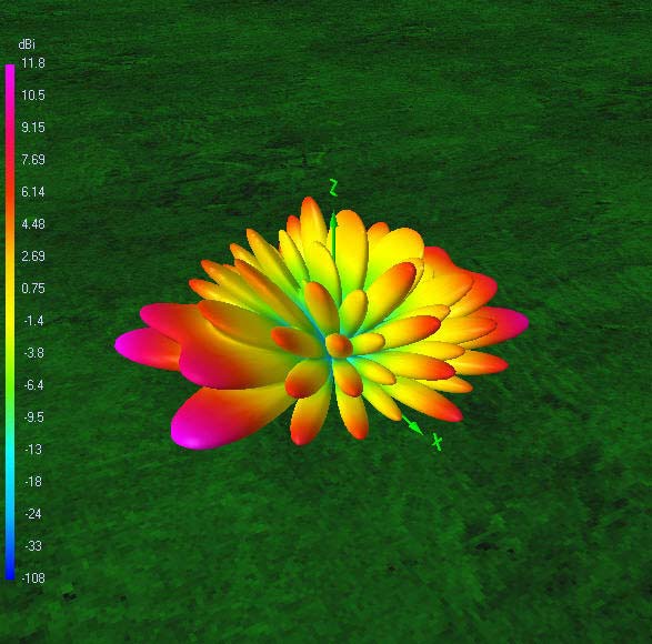
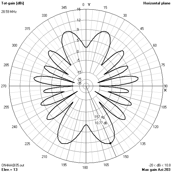
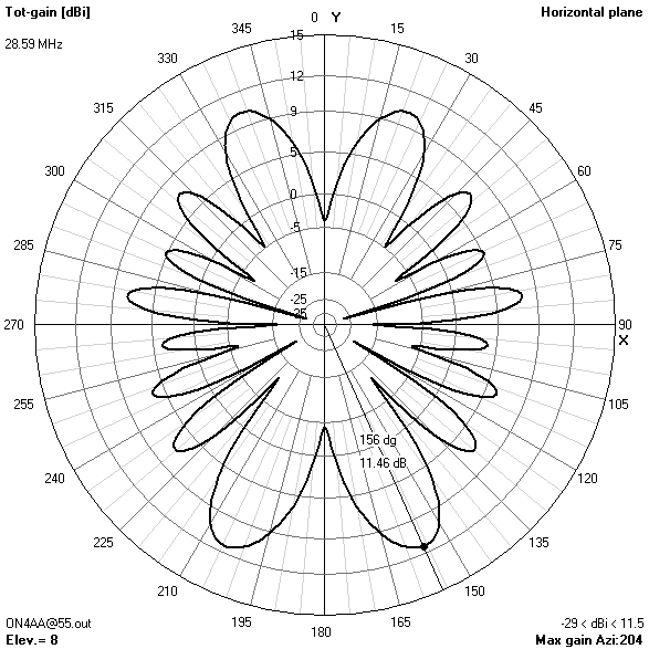
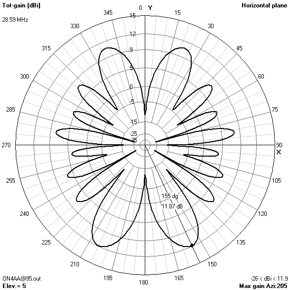
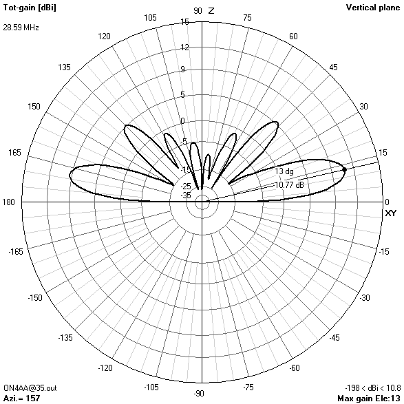
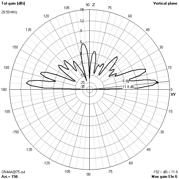
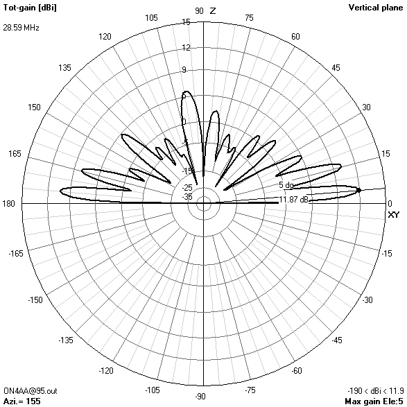
10 m-band radiation patterns
10 m-band or eighth harmonic current distribution
| 10.67 m (35 ft) | 16.76 m (55 ft) | 22.86 m (75 ft) | 28.96 m (95 ft) |
|---|---|---|---|
 \ \ |
 \ \ |
 \ \ |
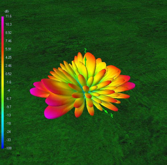 |
| 10.77 dBi ∡ 13° | 11.46 dBi ∡ 8° | 11.80 dBi ∡ 6° | 11.87 dBi ∡ 5° |
 \ \ |
 \ \ |
 \ \ |
 |
 \ \ |
 \ \ |
 \ \ |
 |
Height
Focusing on the lower bands, the most interesting radiation patterns are obtained with an antenna height of about 16.76 m (55 ft). With the antenna at this height:
- On 80 m, the pattern combines maximum gain in the zenith for near-vertical incidence skywave (NVIS) short-haul communications with still enough broadside gain at 30° elevation for long-haul DX contacts.
- On 40 m, a take-off angle of 34° is sufficiently low to enable reliable long-distance (DX) contacts in all directions except for two broadside nulls.
- The 30 m-band is actually the main reason for choosing an antenna height of 16.76 m (55 ft). Only at this height, the useless zenithal lobe will be suppressed.
It is also interesting to see how nulls in certain directions on one band are covered by increased gain lobes on the next harmonic band. This holds true for all six bands. So, one may conclude that the antenna offers spatial diversity through its frequency diversity. Careful selection of operating time and frequency, taking into account available propagation modes, will put you in contact with any place on the globe. This is quite a lot for such a simple, yet very effective, broadband trapless antenna!
A final warning: As with any antenna, be very careful about placing it in the vicinity of other resonant metallic structures (especially antennas) since this may severely upset the desired radiation patterns.
Balun & choke
In theory, the CL-OCFD antenna can be fed with low loss balanced 200 Ω transmission line of any length without any further precautions. Unfortunately, 200 Ω twin line is not commercially available. Moreover, it requires closely spaced wires, which is very hard to construct. If more convenient 50 Ω coax is used as a feed line, the antenna feed point will need to perform three additional tasks:
- Transform the 50 Ω feed line impedance to 200 Ω. This will keep the SWR on the coaxial line below 3÷1, limiting reflection loss and hence eliminating the need to use an open wire feed line.
- Convert the unbalanced currents of the coax to balanced currents, as required by this symmetrically fed antenna. Failing to do so, would severely upset the radiation patterns.
- Prevent both conducted and induced RF currents from flowing back on the outer sheath of the coaxial line towards the shack. Doing so, will eliminate the most common source of radio frequency interference (RFI) occurring with off-center-fed dipole antennas.
Current balun
Tasks 1 & 2 can be performed by a 4÷1 impedance-transforming balun, preferably of the current-type. Voltage type baluns also work, but will be less effective in forcing the right currents on the antenna when nearby metallic objects couple with the antenna. However, do avoid autotransformers or ununs having a common rail between input and output, but lacking a center tap to earth. Here is more information about selecting the right current balun.
A balun for an OCFD needs to to have a high power-rating because it will need to handle the compounded effects of forward power, reflected power and sheath current. The same holds for the sheath current choke. In terms of the power handling capacity as stated on commercial baluns, beware that 1 kW SSB is less than 1 kW CW, is less than 1 kW RTTY, due to the increasing duty cycle of each respective mode. The use of a balun built within a tuner is not recommended because all too often, such baluns happen to be too flimsy. Furthermore, digital modes and FM have duty cycles of up to 100%. This meaning that if you want to operate full legal power in a digital mode, you really would like to have a balun rated at 5 kW CW/SSB.
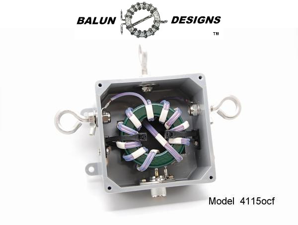
If you happen to live in the USA, I highly recommend dual Guanella element model 4115ocf or hybrid Guanella–Ruthroff model 4116ocf both of Balun Designs. I do not recommend using a single Guanella element on dual core, like model 4114ocf.
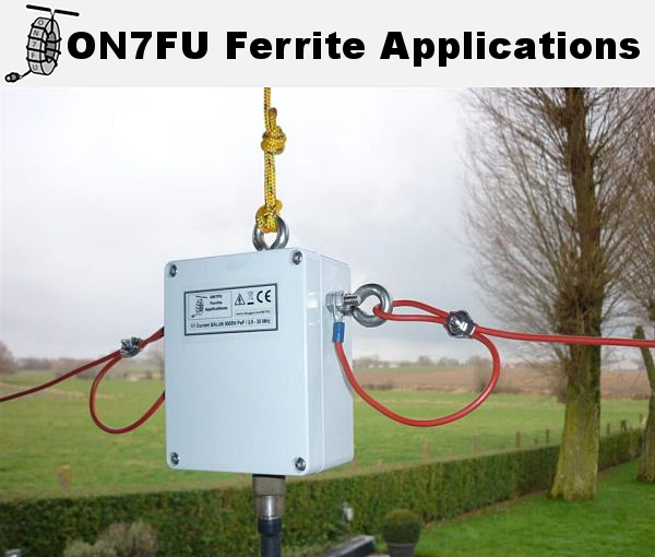
Whereas, prohibitive import taxes render the ON7FU Ferrite Applications 4÷1 dual element Guanella balun a more valuable choice of equal quality for EU citizens.
These baluns are devotedly hand-assembled by respectively Robert J. Rumsey, KZ5R and Hugo Cnudde, ON7FU. I particularly like models with the N-connector option.
Sheath current choke
In many practical realisations of off-center-fed antennas, the third feed point task of preventing the flow of RF currents on the outer sheath of the coax is often overlooked. This is how OCF antennas gained an unfair reputation of being provokers of RFI. Although a current balun will effectively prevent conducted RF currents from flowing along the outer sheath of the coax, it may not always be sufficient to prevent the antenna itself from inducing sheath currents on the coax line. Off-center-fed antennas are more prone to this effect because the coax line is positioned asymmetrically with respect to the antenna.
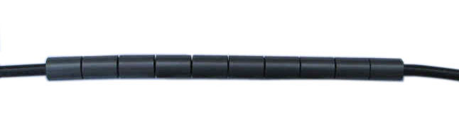
A W2DU sheath current choke prior to applying heat shrink.
Induced sheath currents can easily be prevented. Simply place a sheath current choke right behind the balun. Sheath current choke construction instructions are readily available.
Another sheath current choke may be mounted at the grounded coax bulkhead. This sheath current choke is optional. A coax bulkhead is a grounded metal entry plate through which coaxial lines enter the shack. Such a grounded coax bulkhead is also an excellent lightning protection. It may act as a diversion of last resort for any high currents on the outer sheath of the coax.
Because of their only moderately high sheath impedance, sheath current chokes are only effective when placed at locations where sheath currents require a relatively low impedance to flow. A sheath current choke at any of these locations will introduce, with its lossy magnetic material, a new boundary condition, preventing sheath currents to exist.
Center load components
Capacitor
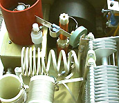
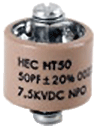 door-knob capacitor
- The table below lists, for an input power of 2500 W, the voltage over the center-loading capacitor at the different operating frequencies.
For the six-band design (220 pF), the highest voltage is 1310 V and is present when the antenna is operated at 10.125 MHz. If the power were only 150 W, the maximum voltage over the 220 pF capacitor would still measure 321 V. At 5 W this would be 59 V. A doorknob capacitor with a voltage rating of at least 2 kV can safely be employed in the six-band design operated at the 2.5 kW power level.
| f (MHz) | U220 pF | U478 pF |
|---|---|---|
| 3.647 | 464 V | ? |
| 7.099 | 62 V | ? |
| 10.125 | 1310 V | — |
| 14.174 | 209 V | ? |
| 21.224 | 403 V | ? |
| 28.594 | 652 V | ? |
Many European surplus doorknob capacitors are Russian made. Picofarad in the Cyrillic alphabet is denoted as пФ. The Cyrillic letter п may appear to Westerners as a Latin n of nano, but in reality it is a Cyrillic “pe” of pico. Kilovolt in Cyrillic is written as кВ. There are more types of high-voltage capacitors; read about them here.
Some have also successfully employed a bank of parallel high-voltage SMD capacitors as a capacitive center load. However, replacing the discrete capacitor with an open stub line would be ill-advised. An open stub line may have the exact same capacitance at its design frequency; on other frequencies it will behave completely differently, upsetting the desired resonances of the antenna.
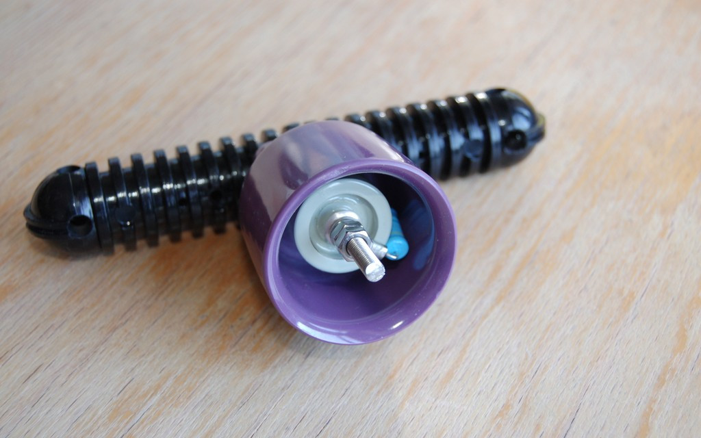
A doorknob capacitor with its snubber resistor installed inside a protective inverted egg cup. The egg cup is made of a durable, weather-resistant plastic. The whole is attached to an antenna insulator.
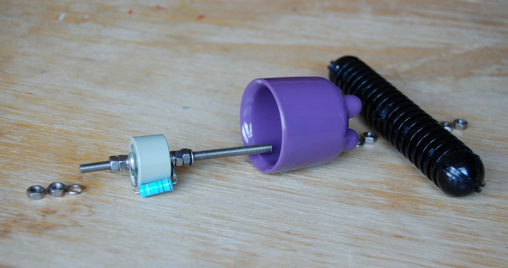
Layout for mounting a doorknob capacitor with its snubber resistor to an antenna insulator. All hardware is A2 stainless steel with an M5 thread.
Snubber resistor
The center-load capacitor C needs to be protected against breakdown from static charges. A 10 kV 1 W thick film metal oxide resistor R of about 1 to 10 MΩ will bleed off any static electricity without incurring any significant loss. Such a protective resistor is also called a snubber.
Inductor
An inductor of 4.95 µH can take on many sizes and shapes. However, the loss and hence quality factor of an inductor will to a certain extent be dependent on its form factor and conductor size. Coils with a form factor that would fit inside a cube often yield the highest quality factor for a given conductor size. Eventually, many designs are a compromise between size, weight and Q factor.
Since I was not satisfied with the accuracy and formulas on which most inductance calculators are based, I designed my own inductance calculator, especially for this project. However, feel free to employ it also for any of your other projects.
Here is a design suggestion for the 4.95 µH center-loading inductor of the six-band CL-OCFD:
According to my inductance calculator, an air coil of length ℓ = 150 mm with a mean diameter D = 150 mm and N = 6.75 turns of diameter 1/4 " (d = 6.35 mm) copper brake pipe will yield an inductance of 4.98 µH at 10.125 MHz; close enough for this application. With these dimensions the unloaded quality factor QL,ul will be a staggering 2220!
The self-resonant frequency of this coil is 31.633 MHz. This is well away from the highest used odd harmonic, 10.125 MHz in this case. (Remember, even harmonics are not influenced by the center-load!)
As for the coil’s construction technique, I prefer AD5X’s plumbing recipe.
Insulators & rope
Insulators
Hams tend to forget about the high RF potentials that are present at the ends of any dipole antenna. Cheap, poor, dirty or broken insulators may form through humid hang ropes an additional path to earth, or at least lower the resonant frequencies. The resistance of such a path may be of the order of mega-ohms. Nevertheless, due to the equally high end-potentials these hidden losses can become quite considerable!
Rope, knots, pulley & weight
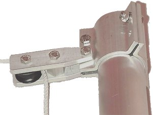 pulley
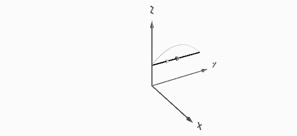
- Horizontal wire antennas are often hung from ropes on both ends. Due to gravitation, flexible wires will hang in the shape of a catenary which corresponds to the graph of a hyperbolic cosine; cosh(x). Considerable tensile forces are required to straighten up the wire a bit. On a stormy day, the wind force may put extra strain on the wire, eventually causing it to snap. A pulley with weight system at one end of the antenna will prevent this from happening. A pulley system will also greatly simplify the trimming of your antenna for resonance as well as general antenna maintenance. Click here for:
- More information on rope types for outdoor use,
- Saving money on stainless steel clamps by knowing some useful knots.
Trimming
How long does the antenna wire need to be?
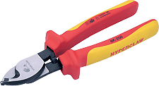 cable cutter
- Above question often returns in many antenna newsgroups. Well, my antenna is actually 40.66 m long, because it is made of 4 mm² gauge PVC-insulated wire and hanging at a height of 16.75 m above a city lot (σ = 1 mS/m; εr = 5). There is a good chance your antenna will end up measuring a different length. It will most probably be hanging at a different height and could be made of another (bare?) wire gauge. Moreover, your location will have different ground characteristics. Look here for a ground-conductivity map of your area. As a result of these influencing factors, your CL-OCFD antenna will probably need to be slightly longer or shorter.
Trimming a wire antenna may seem daunting at first, but as a matter of fact it is absolutely necessary! Any HF antenna —except for a log-periodic— requires element length trimming to compensate for its height above ground. Do not be led fooled by other antenna designs not mentioning this. The need may be less stringent with thick tubing elements, but there are examples abound where it does pay off to even trim very thick elements.9
At what frequency should the antenna wire resonate?
That is a far better question. Here is an universal answer:
The electrical length of the CL-OCFD, at its definitive location and height, should be such that its fundamental resonant frequency is exactly 3.440 MHz. (See the section about resonant lengths). This resonance is measured at the center of the antenna without the center-loading inserted.
Note that this trimming requirement is not exclusively reserved for this antenna. All horizontal HF wire antennas require trimming to adjust to the surroundings. Most manufacturers prefer not to mention this.
The resonance of the antenna wire needs to be checked with the antenna wire at its definitive height and location. The antenna will need to be temporarily fed at its center with the same sheath current choke. This is the very same sheath current choke which will be used later on at a different position along the antenna.
There remains one problem though: How to determine the fundamental resonance of a dipole at 3.440 MHz when it is hanging at a great height above the ground?
At its fundamental resonance, the antenna will have a radiation resistance of 73 Ω. This value coincides with the input impedance when the antenna is temporarily fed at the center. However, when feeding over a test coax of differing characteristic impedance, one will not see resonance even though the antenna is resonating! The happens because the mismatch will add some reactance. See for yourself with AC6LA’s transmission line calculator. Lowering the dipole is neither an option as this will lower its resonant frequency. Here is how to overcome this dilemma…
Using a vector network analyser
Beware! There are little black boxes on the market, pretending to be VNAs. However, many of these little boxes do not offer the possibility to calibrate with a 50 Ω load, a short and an open. If it does not calibrate, is not a vector network analyser! Do not spend any money on this.
A brief guide about using a noise bridge or SWR analyser is available for those not having a VNA at their disposal.
Using a VNA with Bluetooth connectivity
The mini Radio Solutions miniVNA PRO is an affordable vector network analyser (VNA) offering remote wireless operation over Bluetooth. This allows for measuring HF antennas installed at height without having to deal with coax cable lengths, baluns nor common mode suppression chokes. In case of the CL-OCFD, this VNA is able to determine its fundamental resonant frequency at the center, as well as the center load reactance required for resonance on 3.647 and 10.125 MHz. A separate article details how to modify the miniVNA PRO to render it truly field proof.
A modified miniVNA PRO hanging from the center of a HF dipole at about 15 m (50 ft) above ground. A balun is not requiered for taking accurate measurements. The VNA can be read from the comfort of my home even though there are quite some 2,4 GHz WLAN signals present in this urban environment. Two 3350 mAh Panasonic NCR18650B Li-ion cells in parallel provide more than enough «juice» for a whole day of measurements.
Using a VNA with a random length coax line
All what needs to done, is preparing an open (i.e. nothing), a short and a 50 Ω resistive load that can connect to the terminals of the sheath current choke at the end of the random length coax line. If your choke has wire terminals, the 50 Ω calibration load may be constructed out of two high-precision low-inductive 100 Ω resistors. Connect the sheath current choke to a long coax cable and connect the arrangement to the VNA. Hit the calibration button and you are ready to start trimming the antenna at its definitive height.
Trimming procedure
There are two ways of trimming the antenna. The first method was suggested to me by Bob Rose, KC1DSQ. This trimming method requires the antenna wire to be intact at its center. By contrast, the alternative trimming method starts off with the dipole cut at the middle.
Trimming for 7.099 MHz resonance at the 20% feed location
- Start with a slightly too long stretch of antenna wire; say 42 m long.
- Cut the wire at 20%; its intended feed point location.
- Leave the 50% center of the antenna intact.
- Connect a VNA calibrated at 200 Ω at that feed point.
- Trim the antenna for the lowest return loss (SWR) at 7.099 MHz and the other even harmonics; i.e. 14.174 MHz, 21.224 MHz and 28.594 MHz. For each amount of length trimmed off the short end, trim four times that length off the long end.
- Once finished trimming, temporarily reconnect the short and long end.
- Only now, cut the antenna at its 50% center.
- Connect the VNA now at this center location to determine the required reactances for resonance at 3.647 MHz and 10.125 MHz.
The advantage of this approach is that it does not rely on any modelling results (i.e. the 3.44 MHz). All measurements are taken at the frequencies of interest.
Trimming for 3.44 MHz resonance at the center
- Start off with an antenna wire with a length of 42 m. During this process, stick to the rule: «Better having a wire that is too long, than one that is too short!»
- Prepare, as described in the previous section, a half-wave length of test coax (or multiple thereof), resonant at 3.440 MHz. Connect this test coax to the sheath current choke. Alternatively, connect an arbitrary length of test coax to the sheath current choke and calibrate this arrangement with a VNA.
- Cut the antenna wire in the middle. The following may sound too obvious; but for those who do not know: the middle of a long wire is found by folding it in two.
- Connect the test coax with the sheath current choke at the center of the antenna.
- Do not connect the center load nor the balun!
- Hang the antenna at its definitive height and location. Measure the impedance at 3.440 MHz. It should have a positive (i.e. inductive) reactance. This means the antenna is too long for resonance at this frequency. Now, try to find this first lower frequency where the antenna resonates. It should be somewhere below 3.4 MHz. This will give you a feel of what we are looking for at 3.440 MHz. Write down this lower resonant frequency.
- Lower the antenna. —This is why it is handy to have a pulley installed.— Trim off an equal amount of both antenna legs. Use this trimming chart.If you have only one pulley, you may trim the antenna also at its center. Keep note on paper of how much you have been cutting off so far. At this point, the clever wannabes amongst you, would say they can predict how much wire needs to be trimmed off in total. Don’t be fooled in cutting off too much! It is not a linear process, so take it step by step.
- Repeat steps 6 and 7 until you find resonance (reactive part X = 0) at 3.440 MHz. Normally, you should also be able to measure the 7th resonance in the vicinity of 24.912 MHz.
- With the antenna still hanging in the air, measure the reactance at 3.647 MHz and 10.125 MHz. Check if they are more or less equal but opposite in sign of the values listed for XCL at these frequencies. If not, you may want to adapt the values of C and L to your specific case. This only applies to users of VNAs and well-designed noise bridges. Measurements made with SWR analysers are not reliable.
- Now, you may lower the antenna a final time. Remove the sheath current choke from the center.
- Measure 28.9% of the total(!) antenna length and cut the antenna at this point. Take great care in measuring this length accurately, because the VSWR-performance of this antenna is quite sensitive to its relative feed point location. Insert the 4÷1 current balun immediately followed by the sheath current choke at this position.
- Connect the center-loading network at the center of the antenna.
- Raise the antenna, warm up your tube amplifier, tune a little and have fun!
Summary
VSWR performance of ordinary off-center-fed dipoles is always a trade-off between either excellent broad-band performance on 80 m combined with mediocre VSWR on the higher amateur HF bands or vice versa. This problem is due to the fact that the higher amateur HF bands are not true harmonics of the 80 m band.
To overcome this problem, the novel concept of center-loading an off-center-fed dipole (CL-OCFD) is introduced. Center-loading offers indepedent control over a dipole’s fundamental resonant frequency and odd harmonics, whilst off-center feeding ensures low-VSWR coverage of the entire 80 m-band.
Two practical CL-OCFD designs with useful radiation patterns are presented. A five-band design (80, 40, 20, 15 & 10 m) employs a capacitive center-load of 470 pF, whereas a six-band design adds 30 m-band coverage by replacing the center-load by an 4.95 µH inductor in series with a 220 pF capacitor. These designs are not scalable to other bands.
Publications
The center-loaded off-center-fed dipole is the original invention and work of Serge Stroobandt, ON4AA. After its initial publication on the Internet in 2007, the CL-OCFD was subsequently described in the following publications:
Ed Spingola, VA3TPV. Multiband HF antennas, part 3, Windom and OCF dipole. The Communicator. Mississauga; 2010;13(4):9-11. Available at: https://web.archive.org/web/20170518222728/http://www.marc.on.ca/Files/NewsLetters/MARC_NL_2010_04.pdf.
Alois Krischke, DJ0TR, Karl Rothammel†, Antennenbuch. 13th ed.. DARC Verlag GmbH, Baunatal; 2013:301-304. Available at: http://www.antennenbuch.de/.
A year after the online publication of my article, a description of a very similar CL-OCFD for 80 and 160 m was published, equally claiming full 80 m band coverage. There is no reference to my work. It appears to be completely independent work. The antenna is actually a 3-band CL-OCFD antenna (160, 80 & 75 m) where the center loading moves the natural third harmonic to the lower end of the 80 m band, below the 75 m second harmonic.
Gene Preston, K5GP, A broadband 80/160 meter dipole. Available at: https://www.egpreston.com/K5GP_broadband_80_meter_antenna.pdf
References

This work is licensed under a Creative Commons Attribution‑NonCommercial‑ShareAlike 4.0 International License.
Other licensing available on request.

Unless otherwise stated, all originally authored software on this site is licensed under the terms of GNU GPL version 3.
This static web site has no backend database.
Hence, no personal data is collected and GDPR compliance is met.
Moreover, this domain does not set any first party cookies.
All Google ads shown on this web site are, irrespective of your location,
restricted in data processing to meet compliance with the CCPA and GDPR.
However, Google AdSense may set third party cookies for traffic analysis and
use JavaScript to obtain a unique set of browser data.
Your browser can be configured to block third party cookies.
Furthermore, installing an ad blocker like EFF's Privacy Badger
will block the JavaScript of ads.
Google's ad policies can be found here.
transcoded by


 .
.

