VOACAP Primer

James (Jim) Coleman, KA6A

Copyright 1996–2016, licensed under Creative Commons BY-NC-SA

Preface

This text, with the exception of below addendum, first appeared in 1996 as a series of articles on the now defunct site of James E. Mortensen, N2HOS (SK). As an editor, I joined these articles to form one actualised paper, leaving out sections dealing with commercial software that is no longer available. Outdated VOACAP download instructions were deleted and a brief paragraph about VOACAPL was added. (Refer to http://www.voacap.com for up-to-date installation instructions.) Figure 1 has been replaced by a higher resolution picture from the same source. Apart from all that, Jim’s insights remain very instructive and worth reading, even today. Finally, I took the liberty to highlight a number of fragments in benefit of the speed readers among us.

Serge Stroobandt, ON4AA
Hasselt, June 2014

Introduction

The science of radio wave propagation has been developing ever since it was discovered that radio waves somehow went around the earth without simply flying off into space. Everyone who reads the Digital Journal already knows of the impact of HF propagation on commercial, defence, and amateur radio communications. The study of radio wave propagation can constitute a professional career path or a lifelong avocation. Or, as one more example of the great diversity in amateur radio, it can be a topic of the moment for some period of time. But for a ham interested in any aspect of HF operation, digital or otherwise, a basic knowledge of propagation is a most useful tool in the shack.

A great deal of technology has converged in the last few years to make the tool of propagation analysis much more readily available to the radio amateur. Years ago one could only rely on charts in the monthly ham magazines and the updates on WWV at 18 minutes past the hour to make fairly vague analyses of present or future conditions. The professionals over the years have, however, collected much more and better data, and have created better quantitative and analytical models. The decreased cost and increased power of personal computers have made it possible for individual hams to realistically access these better models. And the Internet has made distribution of detailed, nearly real-time data easily available to much larger numbers of hams.

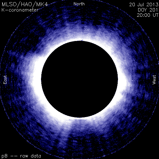
White-light coronameter images from the High Altitude Observatory Mauna Loa Solar Observatory. Source: Solar Data Analysis Center

This paper deals with HF propagation and, in particular, propagation software. The purpose of this paper is not to teach the science of radio wave propagation. That would take a very large introduction and the topic is already adequately covered in a number of fine popular books, textbooks, and university courses on the subject. Our goal here is rather to address radio wave propagation analysis as a tool for the amateur HF operator. We’ll take the practical viewpoint whenever possible and try to get to the nuts and bolts of effectively, and correctly, using software for propagation analysis. We will try to take the point of view of a DX chaser or contester but ask enough of the science to make sure we understand what to put into the software so that what we get out is reliable and useful. Thus, we may not discuss upper atmosphere electron concentrations in any great detail, but we most certainly will discuss signal-to-noise ratios.

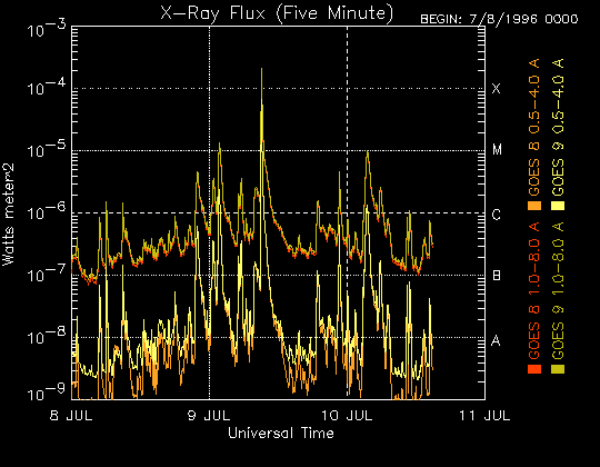
The X-ray Flux plot which shows 3 days of 5-minute solar X-ray flux values measured on the GOES 8 and 9 satellites. Source: NOAA Space Environment Center

Perhaps the most sensible way to introduce the use and capabilities of propagation software is to first frame the question of what each user needs from the analysis and then relate those needs to the science of propagation in a practical way. So let’s get started. For the amateur who is chasing new DX countries, the primary question is pretty straightforward. On what amateur band and at what time can effective signals be exchanged between the two stations. We’ll come back to this most important concept of ‘effective soon.’ For the contester, the primary question is the same except that it isn’t defined in terms of a single DX location — it’s all locations world-wide! For practical reasons it can be at least narrowed to a smaller number of regional locations — say Europe and Asia — and it simply becomes the same exercise multiplied. After that it becomes a matter of contesting strategy.

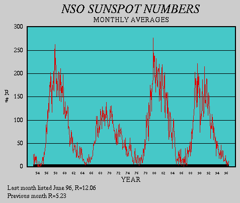
The sunspot number. It is the monthly average R number which is calculated by the following equation: R# = (# of sunspot groups)⋅10 + (# of sunspots). Source: National Solar Observatory

If the main general question is “at what time and at what frequency”, then the first answer that comes to mind is usually MUF, the maximum usable frequency. We are introduced to the concept of MUF, to a greater or lesser extent, quite early in our ham careers. The MUF is indeed a useful concept and can give qualitative insight into propagation. For simplicity, it isn’t all bad to consider the MUF as exactly the answer to our question, provided we are generous with the definition of “exact”. Frequencies well above the MUF are unlikely to be reflected back to earth and those well below the MUF undergo strong absorption or E-layer reflections that make them unusable.

This is all correct, as far as it goes, but calculations of the MUF only tell a part of the story. Actually, the basis for MUF calculations is determined from statistical data on the ionosphere. There are fairly well known relationships between ionospheric parameter and key solar parameter, such as solar flux (sunspots), time of day, season of the year, etc. But, Mother Nature being what she is, the statistical variation is quite large. The MUF is defined as the median value, which means that on any given day there is a 50–50 chance that higher frequency paths will be open.

The MUF has two lesser known cousins — the HPF (highest possible frequency) and FOT (from the French term Frequence Optimale de Travail which is roughly the optimum working frequency). The HPF is the upper limit and can only be exceeded 10% of the time — which is still 3 days a month or 1 day out of a typical 10-day DXpedition. The FOT is defined as 0.85 times the MUF and can be exceeded roughly 90% of the time. The frequency spread between the FOT and the HPF is often 4MHz or more, which is enough to include two different ham bands. So the “required reliability” (i.e. the odds) is something for us to consider.

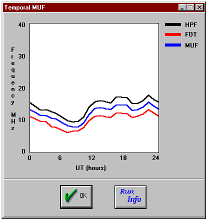
MUF, HPF, and FOT from the HFx software package. Source: Pacific Sierra Research Corporation

Even with statistical considerations aside, MUF calculations don’t give enough information to do the job correctly. Let’s return to the word “effective” for the moment. Effective communications requires that the path be open and that there be distinguishable signals at both ends of the path. Distinguishable means different things under different circumstances. If you are the only station trying to make the contact, then distinguishable implies adequate signal-to-noise ratio, which depends on bandwidth (mode) and things that don’t depend on the ionosphere — like transmitter input power, feedline losses, receiver and transmitter antenna gain profiles, receiver sensitivity and location, and the distance between the receiver and transmitter. It should be easy to see why this problem requires a software solution. In competition with other stations, distinguishable may mean signal-to-interference ratio. For example, if your path to Kermadec from the Midwest US crosses southern California, then noise may matter a lot less than the power output of your California competitors. I’m not aware of any program that calculates signal-to-interference ratio directly but you may need to calculate signal-to-noise ratios for both your path and theirs to determine when your chances are best.

Now we can define the task. The target location must be defined, mode and hardware specified, required probability determined, solar information obtained, and competition identified. Then the software model can be run to determine optimum and backup frequencies and times.

There are other important questions. How is geomagnetic activity treated? For example, many paths from the central US into Asia or the Mideast cross over or through the auroral zone. These signals can be dramatically affected by geomagnetic activity. Are real antenna parameter included? We think of our Yagi antennas as having a certain gain but, in fact, that gain is the peak gain at a certain elevation angle. If the path includes a different arrival angle, and the odds are very good that it will, then a different gain value should be used.

In the next section, I will introduce the basis for many propagation analysis programs — IONCAP (Ionospheric Communications Analysis and Prediction Program) — a program developed originally for mainframes and now ported to higher-power personal computers. Then I will begin our software review with two generations of a program from the Voice of America — VOACAP and VOAWIN.

VOACAP (IONCAP)

In the previous section I introduced a little of the practical aspects of radio wave propagation. Now, we will take a look at a software program (actually a suite of software programs) from the Voice of America (VOA) of the US Department of Commerce. The name of the program is VOACAP and there are two versions. The earlier version, which is now frozen in development and will not be further revised, is a DOS-based program. VOA also released a Windows-based program equally called VOACAP. Development of this software is an ongoing project and new versions of the program are released from time to time.

Jim A. Watson, M0DNS/HZ1JW ported the software to GNU/Linux under the name VOACAPL. Jim also developed pythonProp, a set of tools supporting graphical input and output. Its graphical user interface, evoked by the voacapgui command, permits creation of input files and display of output files.

There are many good reasons to take a good look at VOACAP. One good reason is the price of the program - which is free (unless of course you are a US taxpayer). A second reason is that VOACAP is one of several software packages that are based on a program called IONCAP developed in the late 1970’s by the Institute for Telecommunication Sciences (ITS) of the Department of Commerce. Actually VOACAP and others are “shell” programs that simply act as a user interface for IONCAP and run it for you. IONCAP is probably the best studied propagation program and is arguably the best basis for judging other programs. Thus, we will begin our review of VOACAP with an introduction to IONCAP as seen below.

Since the late thirties, many different organizations have been involved in the study of HF spectrum radio wave communications. A worldwide effort to measure ionospheric parameters, including noise, was established and detailed records have been obtained for variations in system performance over various paths. All of this research has shown that HF system performance is related, in a very complex manner, to solar activity, time of the day, day of the year, and the details of the radio wave path. In 1978, ITS released a FORTRAN program called the Ionospheric Communications Analysis and Prediction Program (IONCAP). Prior to the release of IONCAP, much of the path analysis that was done, had to be handled manually — a very time consuming process. IONCAP was written in a modular format which allowed essentially separate development of models for the key parts of the program.

We won’t go too far into the details of IONCAP, but it is instructive to consider some of them. For example, there are separate subroutines in the IONCAP program for antenna analysis. For any path, the gain of the antenna in the direction of the path and at the elevation angle of the specific signal needs to be considered. In the earliest versions of IONCAP only simple antenna geometries were included but, since it is fairly easy to extend a modular program, VOACAP and other software offer more complex antenna geometries, or the opportunity for you to quantify your own particular antenna system. We’ll talk a little more about this later.

An important subroutine in the IONCAP program is the ionospheric parameter subroutine. Explicit electron density profiles were included in the form of lookup tables, rather than mathematical approximations for these important parameter. But keep in mind that these kinds of approximations are not all bad. The concept of lookup tables for very complex systems can increase computation speed and allows the use of alternate ionospheric models which we will describe a little later in the context of VOACAP.

While IONCAP is the standard for judgement, it isn’t perfect and has some limitations which may, under certain circumstances, be important. For example, IONCAP breaks the year up into twelve months but no further. Thus conditions near the end of the month may look like an average of the results for the present month and the next. IONCAP is designed around the 12-month running average of the sunspot number, not the day-to-day measured solar flux. During sunspot lows, which is the present situation, this doesn’t matter much but near sunspot peaks the differences can be large. IONCAP also does not include geomagnetic effects related to the A- or K-indices. Some of the shell programs, however, do include corrections for this when high latitude paths are involved.

An important and necessary limitation of IONCAP involves paths longer than 10000km — which are often important for DX considerations. The IONCAP single hop model (distances less than 3000km) is very complete and considers all possible ray paths for the circuit. But extension to paths that require three or more hops seldom indicates that there is a path available, which we certainly know to be incorrect. IONCAP uses a correction for these multi-hop paths longer than 10000km. Empirically it has been shown that these circuits are dominated by “control areas” which are the regions within 2000km of either end of the path. If a propagation path does exist, it is because the control area at the transmitter end allows the sky-wave to be launched (first hop) and the control area at the receiver allows what is left of the signal to be returned (last hop). In between, the path can be characterized simply by a loss per distance function and the noise and signal statistics are the same for all paths. This approximation is quite valid and well tested, but implies that one should recognize that the physics is more complete in the model for shorter paths.

When personal computers became powerful enough, IONCAP was incorporated into a form that would run on a PC. The first versions used text input files that mimicked the old FORTRAN punch cards with rigorous requirements on the form and position of the data on each line of input. Output consisted of long printouts of data, also in text format. It didn’t take too long for programmers to create shell programs like VOACAP to make data entry easier and to put the tabular output into a graphical form.

Let’s take a look at VOACAP. Because the DOS version is frozen in development, I’ll only describe the Windows version, but they really aren’t that different. After you download the file named voawin.exe, simply run the program in some temporary directory on your hard drive. Note that a total of more than 26MB of hard drive space is necessary to get the program running. After executing voawin.exe, this directory will have 11.5MB of files in it but you can delete voawin.exe if hard drive space is really critical. Then run install.exe from this temporary directory. The install program will create and fill up a directory called itshfbc (about 14.5MB). The files in the temporary directory can be deleted at this point. You’re done!

The install program will have created a program manager group containing seven programs. There is the usual readme file and a viewer for the collected release notes for VOACAP for Windows called News. There is a program for creating custom antenna profiles called HFANT. VOACAP is the basic point-to-point analysis program, VOAAREA is a version of VOACAP for analysing point-to-area coverage, and S_I VOACAP is a version for calculating signal-to-interference profiles.

VOACAP point-to-point data input

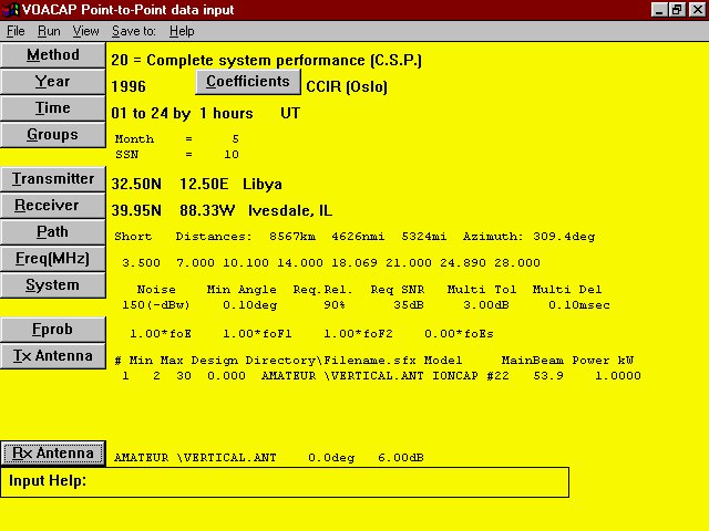
After you’ve launched VOACAP, you’ll get the data input screen shown in Figure 5. All of the input screens have modest balloon style help for the input window corresponding to the mouse pointer. Since most of the input criteria are common to IONCAP-based programs we’ll discuss this screen in some detail. Much of this discussion will also apply to other programs later. IONCAP has a number of different methods but only three of them are commonly used. Method 20 is the complete system performance, method 21 is the same but forces the long path, and method 30 is unique to VOACAP and smooths the transition between the two IONCAP models in the distance range of from 7000–10000km. You have two choices for ionospheric coefficients — CCIR (default) or URSI. We may discuss these in a later article.

The menu choice Groups allows you to choose a number of different months and the associated sunspot number (SSN). This is not the same as the solar flux index given by WWV at 18 minutes past the hour. VOACAP is designed around the 12-month running average of the sunspot number. The average solar flux (SFI) and average sunspot number can be related by

\(SFI = 63.7 + 0.728\cdot SSN + 8.9\cdot 10^{-4}\cdot SSN^2\)

During periods of high solar activity, the running averages can be very different from the daily values while during low activity they don’t differ much. When in doubt, run the program for different values and see what happens.

Transmitter and Receiver can be selected from files called transmit.def and receive.def in the userdb directory. These are text files and can be modified by the user as long as the format is strictly maintained. I have created a set of these files from the CT contest program DX countries database file and will try to find an FTP or web site for those of you who want copies of them. Path can be used to select either short path or long path. Freq(MHz) can be used to select the default short wave frequencies or either of two user-definable frequency lists. These frequencies do not affect the calculations — they only are used for marking the scales on the output graphs.

We only need to concern ourselves with three values under the System prompt. The noise parameter you choose depends on the receiver location. The help menu will give you the information you need to select a value. Required reliability was described last month. 90% is the default and is most useful for contests and DXpeditions but 50% gives you an idea of what may be possible. I usually run the program for both. Required S/N ratio in IONCAP is normalized to a 1Hz bandwidth so the value inserted must include the bandwidth of the receiver which, of course, depends on mode. For SNR use:

\(SNR = 10 + 10\cdot log(BW)\quad \text{where BW is the\ bandwidth in Hz.}\)

A 500Hz bandwidth, CLOVER for example, gives a required SNR of 37dB.

Most users can simply use the default parameter for Fprob. TX Antenna allows up to 4 frequency ranges to be chosen with a different antenna for each. There are 70 different antenna files that can be utilized or the user can create a custom antenna file using the HFANT program described below. Only one RX Antenna can be specified. This may seem a little odd at first but consider that VOACAP was written for broadcast stations not hams. Of course, broadcast stations build complex transmit antenna arrays for specific frequencies and test their systems assuming some basic receiver antenna, such as an isotropic element. From the ham point of view, the choice of antenna and choice of which station is the receiving station is much more complicated. The path between the two stations is not reciprocal, in the sense that you may have different power output at each end. Also, you may not know what kind of antenna the DX is using or even where it’s aimed. I usually assume the basic rule that you have to hear ’em to work ’em and pick KA6A as the RX station. Then I will use realistic receive antennas and guess conservatively on the transmitter antenna and power. Thus, for my purposes, VOACAP would be more convenient to use if it allowed for more RX antennas as well.

VOACAP point-to-point data input

Once the data have been provided, it’s easy to run the program. Simply choose Graph from the Run menu. When execution is completed, you will be given a window full of choices, shown in Figure 6, from which to select the graph output. There is a lot to learn from each of the graphs but, for illustration purposes, look at SNRxx as shown in Figure 7. SNRxx is the signal-to-noise ratio at the probability you specified in the data input window. The solid line is the MUF and the color-coded graph shows you the SNR at any given time and frequency. The horizontal grid lines are the frequencies you specified earlier.

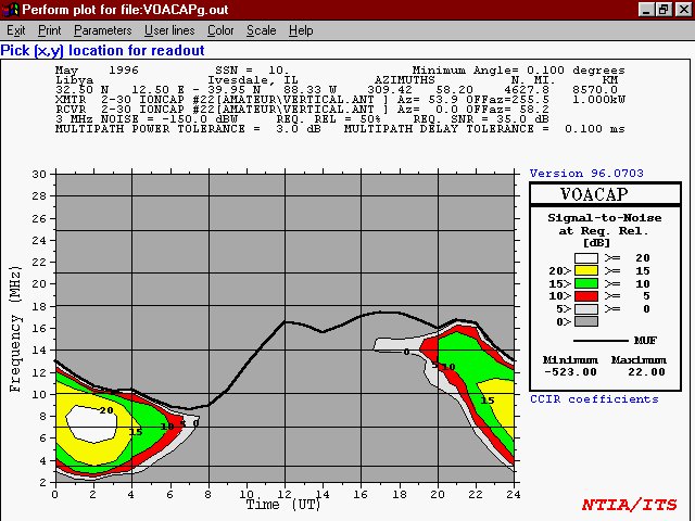
VOACAP signal-to-noise plot at the required reliability of 50%

HFANT data input

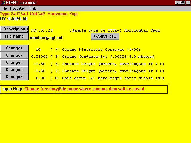
That’s a capsule view of VOACAP. Let’s take a look at the other programs included with the package. The operating window for HFANT is shown in Figure 8. The simplest way to use this program is to open a similar antenna file, modify it however you like, and then use the Save As function to leave the original file unchanged. I created a new directory call Amateur to keep track of my versions. Look at the HFANT plotting capability. It’s great.

VOAAREA is a program that at first glance makes more sense to broadcasters than hams but can be a very useful educational tool for hams. The data input screen is similar to the other VOACAP data input screens. It allows you to specify the transmitter location and the receiver plot center as well as the dimensions of the plot area. An example output window is shown in Figure 9. This is for a transmitter located in Libya and a plot area comprising the continental US. You can see from this graph why we in the Society of Midwest Contesters call the upper Midwest the Black Hole. The SNRs in both 2-land and southern California are 10dB greater than in 9-land!

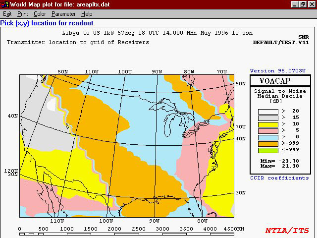
VOAAREA signal-to-noise map plot

The last program in the VOACAP suite is S_I VOACAP, a program that calculates the signal-to-interference ratio. You specify a receiver and two transmitters and the program runs VOACAP for both and automatically calculates interesting interference parameter. This is a brand new part of VOACAP and offers enough potential that I think we’ll cover it by itself in a later column.

The VOACAP suite is powerful and certainly makes a useful tool for analysing radio wave propagation. But there are some weaknesses. The program runs in a reasonable amount of time on a 486-DX2-66MHz machine. A slower machine may be frustratingly slow. This program was developed by a US government agency and, like the government, it has gotten huge. The compressed file is almost 6MB, so downloading it via modem is going to take a long time. Even after the program is completely loaded and temporary files are deleted, it takes almost 15MB of hard drive space! Now, there are a large number of data files included that could be eliminated, but that takes time and some experience with the program. I’ve already mentioned that geomagnetic activity is not considered. In fact, the readme file explicitly warns against using VOACAP for short term prediction. It can indeed be used for short term predictions, of course, as long as you understand the limitations. I have a mixed opinion of the graphics. The colour scale 3-dimensional graphs work fine on the screen but do not lend themselves to black and white printing. A black and white switch is included in the program but the results are unimpressive. The program does not have single band output graphs — a feature I think is important.

My overall recommendation? C’mon… the program is free! Seriously, if you have the disk space and a reasonably powerful machine, this one is worth getting and using. Is it the best program available? Other programs do some things better, even much better in some cases, but all things considered (including price) this might indeed be the best program available.

Next time we’ll look at another IONCAP shell program called CAPMAN. If you have any specific questions related to radio wave propagation, send them to me and I’ll try to answer them either as a short answer at the end of one of these articles or as the basis for a later article. And, as usual, if I don’t know the answer, I’ll try to make up something plausible. Hi!

Contest planning

I thought it might be interesting to address propagation also from a contest planning point of view. Needless to say, my perspective will be heavily weighted toward operation from the area referred to, by the Society of Midwest Contesters, as the “Black Hole” — Wisconsin, northern Illinois, eastern Iowa and western Indiana. In order to decide what to look for from propagation analysis, we need first to define the problem. Let’s assume that the operation is defined as shown in Table 1.

Contest parameters
Contest	Any DX contest (no value in W/VE QSOs)
Bands	All
Transmitters	Single
Power	High
Antennas	Rotatable beams on 7MHz and higher, wires elsewhere

Thus, given the usual propagation parameter of solar flux and geomagnetic activity, we need to determine a beam heading and frequency for any time period in the 48 hours of the contest. There are additional constraints, of course. We want to maximize our score which means we want to have the maximum number of QSOs and the maximum number of multipliers. We’ll look at these separately. Finally, we need to be concerned about the competition, although we can also learn a lot in real time from our competition.

Let’s look at maximizing QSOs. Anywhere in the US, maximizing QSOs means concentrating on Europe and Japan, where the densities of contesting hams are the highest. And unless band conditions are very good, Japan is a distant second for the Midwest and the east coast. So in terms of running stations, our first priority will be to key on these two regions of the world. Europe is, of course, a very large area taken as a whole and, though you might not want to take time to do it during the contest, it is interesting to observe how the propagation in the morning from Europe begins with Scandinavia first and progresses through to southeastern Europe and the Balkans. After these two regions, perhaps South America is the next most active region during a contest, but the numbers of active contesters just can’t match Europe or Japan.

In terms of the region with greatest density of country multipliers, it might be a toss up between Europe, which consists of many countries and a large number of active ham contesters, and the Caribbean, which consists of a surprisingly large number of very small countries, most of which are activated by contest teams launching large multi-multi efforts. From a propagation point of view, both of these sources of country multipliers are no-brainers. First, for QSO purposes we plan on strongly emphasizing Europe anyway and there usually isn’t a strong need to search for new multipliers from Europe. The obvious exception to this is very rare European countries, such as the Sovereign Military Order of the Knights of Malta, that occasionally mount a strong contest effort. The reason that the Caribbean is a no-brainer is simply that propagation windows to the Caribbean are generally wide on all bands, the signals are strong even with poorer propagation conditions, and the operators of those efforts are usually superb. There is no excuse for not working every Caribbean country on every band in every contest. After these two regions, however, multiplier hunting becomes a more difficult problem and is an exercise involving some elements of luck, skill, and rotator fatigue.

What about the competition? From the Midwest, the competition to Europe is the east coast, of course. For the most part, there is only a brief period when the east coast has Europe while they cannot be heard in the Midwest. The paths and path lengths just aren’t that different. There are enough stations for everyone to maintain pretty respectable rates. The competition from the western US for JA stations can be much more frustrating. The openings to Japan are much longer for western US stations, and contesters in the Midwest can listen for long periods of time to stations like W0UN running JA stations without actually hearing any of the JA station themselves. I’m sure the frustration is even greater for east coast contesters, especially if the polar paths are disturbed.

So how do you use this competition to your advantage? The fastest way to learn about conditions to any region is to listen to the stations that the competition is working and consider the rate at which they are being worked. It may just tell you stay on the band or move to a different band.

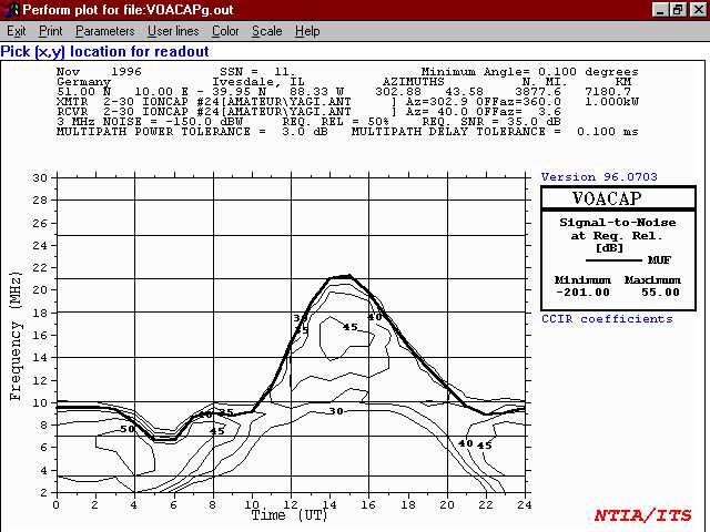
Propagation from the Midwest US to Germany with a reliability of 50%

Okay, let’s look at some examples. Figure 10 shows the propagation from the Midwest US to Germany. This particular plot is from VOACAP for Windows and is the signal-to-noise-ratio at the required reliability (50%). The most basic approach to band selection involves considering the MUF (solid line) to be a band about 3MHz wide. The plots indicate that we will probably get nothing on 10 meter, which is no surprise at this point in the sunspot cycle. The opening on 15 meter is likely not too long - perhaps a few hours around 1400Z. 20 meter looks good from as early as 1100 or 1130Z to as late as 2000Z. The rest of the time would be mainly spent on 40 meter, broadcast stations permitting, with a brief shot at 80 or 160 around 0500Z. Keep in mind the relative statistical basis of propagation prediction and use your ears more than the computer.

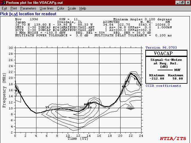
Propagation from the Midwest US to Japan with a reliability of 50%

The situation for Japan is more depressing. Figure 11 shows the VOACAP for Windows signal-to-noise-ratio at the required reliability (50%) from the Midwest US to Japan. The 20 and 15 meter openings are much narrower in time. The MUF stays relatively high, which means that 40 meter absorption may limit openings on that band to a short time around 1200Z. If the geomagnetic activity is high, polar absorption, which is important for the Midwest US to Japan path, may dominate. An easily possible result is a 40 minute opening to Japan on 20 meter and little else. Contesting can be more fun during sunspot peaks, if not more challenging!

What about the rest of the world? It’s much harder to be specific. The afternoon hours local time (1800-2100Z) are good times to look for multipliers from Africa, the south Atlantic, and South America but the rates are usually pretty low. In the later evening local time, after the Japan window closes on the upper bands, it would be good to look at south Pacific and VK/ZL openings. These are usually weaker signals and the beam headings are unique so you may not hear anything unless you actively go after them. Of course, you don’t want to miss any opportunity to work any of the Caribbean contest teams. In any case, we are searching for multipliers so a lot of tuning, listening, and beam spinning is necessary. I usually work up an hour-by-hour band and beam heading plan with some specific options for hours when there is more than one possibility. After the contest, you can compare the plan with your actual rates to specific areas and fine tune the planning process for the next big contest.

All of this discussion was designed around active participation in a multi-band effort. If your real interest is understanding propagation and you are less enthusiastic about contesting, contest weekends still offer the opportunity for an amazing real-world laboratory experiment. Here are two example experiments. For the first example, choose a single band, like 15 meter, and then observe the contesting stations locations and signal strengths. You can simply monitor the band for a few minutes every hour. Spots broadcast on your local DX cluster node can be a great help for this experiment. Then compare the observed data with those predicted by your favourite program. In the second experiment, choose a single location, like western Europe, and hour-by-hour track signals from a single specific country on each band. Then make the same comparison with your software. Either of these experiments could be done as a participant or silent observer in the contest. And you’ll learn more in a single weekend than you can otherwise in a much longer period of time.

Well that’s it. Look for either KA6A or K9USA in any of the CW or RTTY contests.

Addendum

From: k6sti at n2.net (Brian Beezley)
Date: Tue, 9 Apr 1996 20:13:32 -0700
Subject: VOACAP
Message-ID: <199604100313.UAA15858 at ravel.n2.net>

I’d like to alert contesters to the fabulous VOACAP propagation-prediction program available for free at ftp.voa.gov. This is a version of the professional IONCAP program that has been substantially enhanced for use by the Voice of America on HF circuits.

Here’s what you can do with VOACAP: Specify the month of the year, the sunspot number, your QTH, power, antenna type, height above ground, and many other station parameter. Define an area of interest (Europe, for example). VOACAP then draws a map of the area with receive signal strength, S/N, MUF, radiation angle, or any of a dozen other parameter overlaid as continuous colour regions. You can see your coverage area at a glance. You can change any parameter and see how it affects coverage. The graphics are stunning and the information fascinating.

I think every serious contester should have a copy of VOACAP. It’s a tremendous tool both for investigating unknown but possible DX paths and for checking your coverage into high-rate regions. For example, Dean Straw, N6BV, checked his coverage into Europe by plotting signal-strength maps. The maps revealed unexpected coverage holes in localized but high-population areas due to pattern nulls in his antenna system. There’s simply no other way to obtain valuable information like this. Get the Windows version — the DOS version lacks certain features and will not be developed further.

To increase VOACAP prediction accuracy, I’ve written a little utility to convert elevation patterns generated by the TA 1.0 Terrain Analyzer program to VOACAP antenna files. This utility lets you generate VOACAP maps using the elevation pattern of your specific antenna system as sited in your local terrain. If you have TA and would like a copy of this utility, I’ll be happy to e-mail it to you. Please specify uuencode, MIME, or BinHex format.

73 — Brian, K6STI
k6sti at n2.net

This work is licensed under a Creative Commons Attribution‑NonCommercial‑ShareAlike 4.0 International License.
Other licensing available on request.

Unless otherwise stated, all originally authored software on this site is licensed under the terms of GNU GPL version 3.

This static web site has no backend database.
Hence, no personal data is collected and GDPR compliance is met.
Moreover, this domain does not set any first party cookies.

All Google ads shown on this web site are, irrespective of your location,
restricted in data processing to meet compliance with the CCPA and GDPR.
However, Google AdSense may set third party cookies for traffic analysis and
use JavaScript to obtain a unique set of browser data.
Your browser can be configured to block third party cookies.
Furthermore, installing an ad blocker like EFF's Privacy Badger
will block the JavaScript of ads.
Google's ad policies can be found here.

This page employs a