
RF Inductance Calculator for Single‑Layer Helical Round‑Wire Coils
Serge Y. Stroobandt, ON4AA
Copyright 2007–2020, licensed under Creative Commons BY-NC-SA
- Home
- Inductance Calculator

Copy & paste
Achieving a high quality factor
Coils achieving the highest quality factor require large diameter wire, strip or tubing and usually exhibit a cubical form factor; i.e. the coil length equals the coil diameter.
Frequently asked questions
In what does this inductance calculator differ from the rest?
 Dr. James F. Corum, K1AON
- The inductor calculator presented on this page is unique in that it employs the n = 0 sheath helix waveguide mode to determine the inductance of a coil, irrespective of its electrical length. Unlike quasistatic inductance calculators, this RF inductance calculator allows for more accurate inductance predictions at high frequencies by including the transmission line effects apparent with longer coils. Furthermore, the calculator closely follows the National Institute of Standards and Technology (NIST) methodology for applying round wire and non-uniformity correction factors and takes into account both the proximity effect and the skin effect.
The development of this calculator has been primarily based on a 2001 IEEE Microwave Review article by the Corum brothers7 and the correction formulas presented in David Knight’s, G3YNH, theoretical overview,1 extended with a couple of personal additions.
Which equivalent circuit should be used?
Both equivalent circuits yield exactly the same coil impedance at the design frequency.
For narrowband applications around a single design frequency the effective equivalent circuit may be used. When needed, additional equivalent circuits may be calculated for additional design frequencies.
The lumped equivalent circuit is given here mainly for the purpose of comparing with other calculators. By adding a lumped stray capacitance in parallel, this equivalent circuit tries to mimic the frequency response of the coil impedance. This will be accurate only for a limited band of frequencies centred around the design frequency.
What can this calculator be used for?
 helical antenna
- The calculator returns values for the axial propagation factor β and characteristic impedance Zc of the n = 0 (T0) sheath helix waveguide mode for any helix dimensions at any frequency.
This information is useful for designing:
- High-Q loading coils for antenna size reduction (construction details),
- Single or multi-loop reception antennas with known resonant frequency,
- Helical antennas, which are equivalent to a dielectric rod antenna,
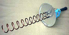
- Tesla coil high-voltage sources (see picture further on),
- RF coils for Magnetic Resonance Imaging (MRI),
- Travelling wave tube (TWT) helices (picture below).
What is the problem with other inductor calculators?
 Tom Rauch, W8JI
- Tom Rauch, W8JI, in his well-known high-Q inductor study once complained that many inductor modelling programs fail to consider two important effects:
- The stray capacitance across the inductor,
- The proximity effect, causing Q to decrease as turns are brought closer together.
For example, the RF Coil Design JavaScript calculator by VE3KL ignores these effects.
Likewise, a once very popular computer program, named «COIL» by Brian Beezley ex-K6STI happened to be based on a set of faulty formulas,1,10,11 as has been carefully pointed out by David Knight, G3YNH. The program is luckily no longer commercially available.
How is the helical waveguide mode being calculated?
 Friedrich Wilhelm Bessel
- A coil can be best seen as a helical waveguide with a kind of helical surface wave propagating along it. The phase propagation velocity of such a helical waveguide is dispersive, meaning it is different for different frequencies. (This is not the case with ordinary transmission lines like coax or open wire.) Lower frequencies propagate slower along a coil. The actual phase velocity at a specific frequency for a specific wave mode is obtained by solving a transcendental eigenvalue equation involving modified Bessel functions of the first (In) and second kind (Kn) for, respectively, the inside and the outside of the helix.7,8
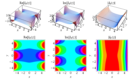
Modified Bessel function of the first kind, order 0; solution to the field inside the helix. Source: Wolfram Mathworld
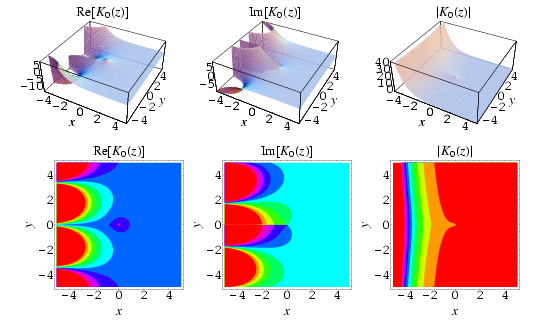
Modified Bessel function of the second kind, order 0; solution to the field outside the helix. Source: Wolfram Mathworld
 Dr T. J. Dekker
- Since such an equation cannot be solved by ordinary analytical means, the present calculator will determine the phase velocity β of the lowest order (n = 0) sheath helix mode at the design frequency using Theodorus (Dirk) J. Dekker’s12–14 combined bisection-secant numerical root finding technique. For this calculator, a SLATEC FORTRAN version15 of Dekker’s algorithm was translated by David Binner to JavaScript code, and then from there by yours truly to Brython code.
A similar algorithm is also employed to home in on the frequency for which the coil appears as a quarter wave resonator. This is the first self-resonant frequency of the coil.
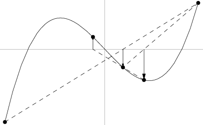
The secant root finding method. Source: Wolfram Mathworld
More details about the employed formulas and algorithms can be obtained immediately from the Brython source code of this calculator.
Why are correction factors still needed?
Even though the sheath helix waveguide model is the most accurate model available to date, it certainly suffers from a number of limitations. These have their origin in the very definition of a sheath helix, being: an idealised anisotropically conducting cylindrical surface that conducts only in the helical direction.7
By choosing a sheath helix as the model for a cylindrical round wire coil, the following assumptions are made:
- The wire is perfectly conducting.
- The wire is infinitesimal thin.
- The coil´s turns are infinitely closed-spaced.
- Finally, since higher (n > 0) sheath helix waveguide modes are disregarded, end effects in the form of field non-uniformities are not dealt with. Hence, the sheath helix needs to be assumed to be very long and relatively thin in order for the end effects to become negligible.
- Luckily, these assumptions happen to be identical to the assumptions made when using a geometrical inductance formula. This implies that the very same correction factors may be applied to the results of the sheath helix waveguide model, being:
- A field non-uniformity correction factor kL according to Lundin1,3 for modelling the end-effects of short & thick coils (high \(\frac{D}{\ell}\) ratio),
- A round wire self-inductance correction factor ks according to Rosa,1,4,5
- A round wire mutual-inductance correction factor km according to Knight,1,6
- A reduced effective coil diameter for modelling the current quenching in the wire under the proximity effect of nearby windings,
- A series AC resistance for modelling the skin effect including an additional end-correction for the two end-turns that are subject to only half the proximity effect.
Is there a small discontinuity in calculated inductances?
Yes, there is; around ℓ = D. Thomas Bruhns, K7ITM discovered this little flaw. It is entirely due to the intrinsically discontinuous formulation of Lundin’s handbook formula. This approximative formula is used to obtain the field non-uniformity correction factor kL without much computational burden. The discontinuity in calculated inductances appears only whenever ℓ = D. It is only pronounced when the sum of the correction factors (ks + km) is relatively small in comparison to kL; i.e. for really thick, closed-spaced turns. However, even then, the error is not larger than ±0.0003%.1
Are there any other approximations being made?
 Dr David W. Knight, G3YNH
- Yes, there are a few other approximations. These are introduced only when the computational gain is substantional and when the impact on accuracy is less than any feasible manufacturing tolerance. Apart from the previously discussed Lundin’s handbook formula, David Knight’s approximation formula1 is employed to determine the correction factor km for round wire mutual inductance.1 The effective diameter Deff is also being estimated, simply because there is currently no known way to calculate it (see below).
Does this calculator rely on any empirical data?
The proximity factor Φ, used for calculating the AC resistance of the coil, is interpolated from Medhurst’s table of experimental data.2 The proximity factor Φ is defined as the ratio of total AC resistance including the contribution of the proximity effect over AC resistance without the contribution of the proximity effect.
\[\Phi \equiv \frac{R_{ac,\Phi}}{R_{ac}}\]
How is the effective diameter Deff related to the proximity factor Φ?
Other inductor calculators typically employ the mean and inner physical diameters (respectively: D and D - d) to bracket the inductance of the coil between two widely spaced theoretical limits1. However, it has often been alluded that the actual effective diameter Deff of a coil aught to be linked to the proximity factor Φ. In order to do away with the ambiguity of an inductance range result, a novel, naive approximation formula was deduced. With this approximation, the effective diameter Deff is a mere function of the proximity factor Φ. As a result of this effort, this inductance calculator will return only a single value of inductance.
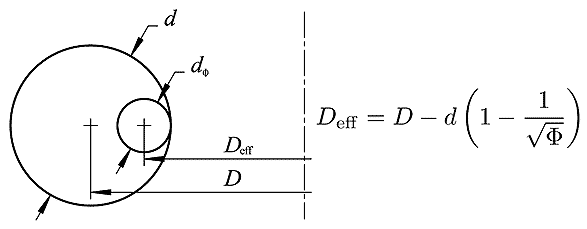
The effective diameter and its presumed relation to the proximity factor Φ (see text)
Although being more specific than effective diameter bracketing, inductance calculations based on this formula remain approximative for two reasons:
- As is the case with diameter bracketing, this formula equally assumes that current under the proximity effect will quench while retaining a circular transversal distribution. This is most probably not the case.
- As with diameter bracketing, the formula does not take into account frequency dependent disturbances of the transversal current distribution, such as the skin effect.
These disturbances in transversal current distribution are not accounted for and may move the current distribution centre further inward. This reduces the effective diameter and, by consequence, the inductance even more. The inductance obtained by this calculator will therefore be slightly overstated. Nonetheless, the reported inductance will in most circumstances result more accurate and certainly less ambiguous than the theoretical extremes (or average thereof) given by other inductance calculators.
The inductance, and hence the Q-factor, near resonance are enormous; Can this be right?
As explained before, the correct way to see an inductor is as a helical waveguide, short-circuited at one end —because it is assumed to be fed with a voltage source. At any frequency, the axial propagation factor β and the characteristic impedance Zc of an equivalent transmission line can be determined.
The input impedance seen at the other end will be a tangential function of the coil’s electrical length. Therefore, when the electrical length approaches a quarter wave length or \(\frac{\pi}{2}\) rad, the resulting input impedance, and hence the inductance, will be extremely high. The ohmic losses remain comparatively low, so the quality factor Q will be huge near resonance.
A Tesla coil employs this phenomenon to produce extremely high voltages in the range of several hundreds of kV.7 Inductance calculators that do not show this real world behaviour are based on geometrical formulas.
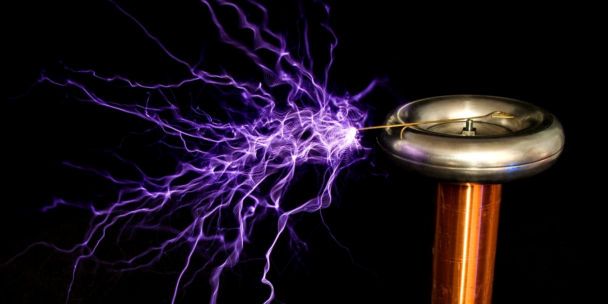
Voltage breakdown of the air at one end of a Tesla coil. Source: oneTesla
The calculated inductance is negative; Can this be right?
You are operating the coil above its first self-resonant frequency. A coil with an electrical length in-between 90° and 180° (and odd multiples of this) will behave like a capacitor instead of an inductor. This is once more an indication that the first self-resonance of a coil is in fact a parallel resonance. Because of its capacitive behaviour, the coil’s inductance will be stated as negative in this range.
Stray capacitance Cp is much higher than that of other calculators; Can this be right?
The concept of stray capacitance is what it is; a correction element in a coil’s lumped circuit equivalent to deal with the frequency independence of an inferior geometrical inductance formula.7
By employing helical waveguide-based formulas, the present calculator performs much better at estimating inductances at high frequencies. Therefore, the calculator compensates the lumped circuit equivalent even more so than other calculators. This results in higher values for Cp.
At the end of the day, the old-fashioned concept of a lumped circuit equivalent is better done away with. Instead, focus on the effective values at the design frequency for inductance, reactance, series resistance and unloaded Q.
What is the problem with designing coils using EZNEC?
The pragmatists among us would probably like to employ EZNEC, an antenna modelling program, which allows you to define in a very user-friendly way helical coil structures. However, this valuable method is not without its pitfalls:
- Coils in EZNEC are defined as polyline structures. The projected polygon of the polyline should have the same area as the projected circle of the real helical coil. I will leave it up to the reader to perform this trigonometric exercise.
- The more segments in the polyline, the more accurate the model would represent the real helical coil. However, EZNEC has a lower limit for the segment length which is proportional to the wavelength.
- In view of the two previous points, it is quite cumbersome to optimise a coil design using EZNEC.
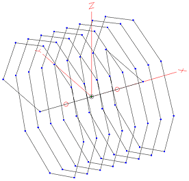
EZNEC coil model
In practice, it is often much easier, quicker and more accurate to resort to the above calculator instead of creating a geometrical EZNEC coil model. Once the results are obtained from this calculator, the coil can be easily modelled as a Laplace load within any EZNEC antenna model.
Formulas
The winding pitch of a single-layer coil is defined as
\[\begin{equation} p \equiv \frac{\ell}{N} \end{equation}\]
The proximity factor \(\Phi\) is interpolated from empirical Medhurst data.1,2
\[\begin{equation} \Phi=f_\text{Medhurst}\left(\frac{\ell}{D},\frac{p}{d}\right) \end{equation}\]
A naive, approximative formula for the effective diameter \(D_\text{eff}\) was deduced by the author:
\[\begin{equation} D_\text{eff} = D - d \cdot \left(1 - \frac{1}{\sqrt{\Phi}}\right) \end{equation}\]
Correction factors
\(k_\text{L}\) is the field non-uniformity correction factor according to Lundin.1,3 Under the stated condition, the short coil expression is a better approximation to Bob Weaver’s arithmetico-geometric mean (AGM) method than the long coil expression.1
For short coils \(\ell \leqslant D_\text{eff}\):
\[\begin{equation}\begin{split} k_\text{L} = \frac{2\ell}{\pi D_\text{eff}}\;\left[ \frac{1 + 0.383901\;\left(\frac{\ell}{D_\text{eff}}\right)^2 + 0.017108\;\left(\frac{\ell}{D_\text{eff}}\right)^4}{1 + 0.258952\;\left(\frac{\ell}{D_\text{eff}}\right)^2}\;\left[\ln{\frac{4D_\text{eff}}{\ell}} - 0.5\right]\\ + 0.093842\;\left(\frac{\ell}{D_\text{eff}}\right)^2 + 0.002029\;\left(\frac{\ell}{D_\text{eff}}\right)^4 - 0.000801\;\left(\frac{\ell}{D_\text{eff}}\right)^6 \right] \end{split}\end{equation}\]
For long coils \(\ell > D_\text{eff}\):
\[\begin{equation} k_\text{L} = \frac{1 + 0.383901\;\left(\frac{D_\text{eff}}{\ell}\right)^2 + 0.017108\;\left(\frac{D_\text{eff}}{\ell}\right)^4}{1 + 0.258952\;\left(\frac{D_\text{eff}}{\ell}\right)^2} - \frac{4D_\text{eff}}{3\pi\ell} \end{equation}\]
\(k_\text{s}\) is the correction factor for the self-inductance of the round conductor according to Knight and Rosa.1,4,5
\[k_\text{s} = \frac{5}{4} - \ln{\left(2\,\frac{p}{d}\right)}\]
\(k_{\text{m}}\) is the correction factor for the mutual-inductance between the round conductor windings according to Knight.1,6
\[k_{\text{m}} = \ln{(2\pi)} - \frac{3}{2} - \frac{\ln{(N)}}{6N} - \frac{0.33084236}{N} - \frac{1}{120N^3} + \frac{1}{504N^5} - \frac{0.0011925}{N^7} + \frac{c_9}{N^9}\]
where \(c_9 = -\ln{(2\pi)} +\frac{3}{2} +0.33084236 +\frac{1}{120} -\frac{1}{504} +0.0011925\)
Effective series AC resistance
The physical and effective wire or tube conductor lengths derived from Pythagoras’ theorem:
\[\ell_\text{w,phys} = \sqrt{(N \pi D)^2 + \ell^2}\]
\[\ell_\text{w,eff} = \sqrt{(N \pi\,D_\text{eff})^2 + \ell^2}\]
The skin depth \(\delta_\text{i}\) at the design frequency \(f\) is given by:9
\[\delta_\text{i} = \sqrt{ \frac{\rho}{\pi f \mu_0\,\mu_\text{r,w}} }\]
At the design frequency, the effective series AC resistance \(R_{\text{eff,s}}\) of the round wire coil is:9
\[R_{\text{eff,s}} = \frac{\rho\;\:\ell_\text{w,eff}}{\pi\,(d\,\delta_\text{i} - \delta_\text{i}^2)}\,\Phi\,\frac{N - 1}{N}\]
For a single loop, the proximity end correction factor \(\frac{N - 1}{N}\) in above formula is replaced by a factor 1.
Corrected current-sheet geometrical formula
The frequency-independent series inductance \(L_{\text{s}}\) from the current-sheet coil geometrical formula, corrected for field non-uniformity and round conductor self‑inductance and mutual coupling is:1,3–6
\[L_\text{s} = \mu_0\left[\pi\frac{(D_\text{eff} N)^2}{4\ell} - D_\text{eff} N\frac{k_\text{s} + k_\text{m}}{2}\right]\]
Characteristic impedance of the sheath helix waveguide mode
The effective pitch angle is calculated from trigonometry:
\[\psi = \arctan{\frac{p}{\pi\,D_\text{eff}}}\]
It was shown by Hertz that an arbitrary electromagnetic field in a source free homogeneous linear isotropic medium can be defined in terms of a single vector potential \(\Pi\).16 Assuming \(\,\text{e}^{\,\text{j}\omega t}\) time dependency, a wave in the Hertz vector potential field can be written as:
\[\vec{\Pi}(x) = \vec{\Pi}(0) \,\text{e}^{-\gamma x}\]
The propagation constant \(\gamma\) is a complex quantity:
\[\gamma = \alpha + \text{j}\beta\]
\(\alpha\) is the attenuation constant, and
\(\beta\) is the phase constant.
However, since the attenuation in an air medium is negligible, it is customary to write the wave equation solely in function of a complex phase constant \(\beta\):
\[\vec{\Pi}(x) = \vec{\Pi}(0) \,\text{e}^{-\text{j}\beta x}\]
such that \(\gamma \equiv \text{j}\beta = \text{j}(\beta' -\text{j}\beta'') = \beta'' + \text{j}\beta' \Rightarrow \beta'' \equiv \alpha\).
Separation of variables in the Helmholtz equation results in a transcendental sheath helix dispersion function7 that needs to be solved numerically for the transverse (radial) wave number \(\tau\):
\[{k_0}^2 \frac{ \text{K}_1(\tau a)\;\text{I}_1(\tau a) }{ \text{K}_0(\tau a)\;\text{I}_0(\tau a) } = \tau^2 \tan^2(\psi)\]
the effective radius \(a = \frac{D_\text{eff}}{2}\),
the free space angular wave number \({k_0} \equiv \frac{\omega}{c_0} = \frac{2\pi}{\lambda_0}\), and
the transversal wave number \(\tau^2 = -\left(\gamma^2 + {k_0}^2\right) = \beta^2 - {k_0}^2\)
\[\Rightarrow \beta = \sqrt{{k_0}^2 + \tau^2}\]
The characteristic impedance \(Z_\text{c}\) of the \(n = 0\) sheath helix waveguide mode at the design frequency is given by:7
\[Z_\text{c} = \frac{60\beta}{k_0}\,\text{I}_0(\tau a)\;\text{K}_0(\tau a)\]
Corrected sheath helix waveguide formula
\[L_\text{eff,s} = \frac{Z_\text{c}}{\omega}\,\tan(\beta\,\ell)\;k_\text{L} - \mu_0 D_\text{eff} N\frac{k_\text{s} + k_\text{m}}{2}\]
Effective equivalent circuit
\[X_\text{eff,s} = \omega L_\text{eff,s}\]
\[Q_\text{eff} \equiv \frac{X_\text{eff,s}}{R_\text{eff,s}}\]
Lumped equivalent circuit
To calculate the lumped equivalent circuit, first the known series effective equivalent circuit is converted to its parallel version:
\[R_\text{eff,p} = \left(Q_\text{eff}^2 + 1\right) R_\text{eff,s} \qquad X_\text{eff,p} = \frac{Q_\text{eff}^2 + 1}{Q_\text{eff}^2} X_\text{eff,s}\]
Likewise, the lumped equivalent circuit can be converted to a circuit with only parallel components, in which \(Q_L\) and \(R_\text{s}\) remain unknown:
\[R_\text{p} = \left(Q_L^2 + 1\right) R_\text{s} \qquad X_{L_\text{p}} = \frac{Q_L^2 + 1}{Q_L^2} X_{L_\text{s}}\]
Three more identities can be written; the first states that the parallel resistors in both equivalent circuits are one and the same:
\[R_\text{p} = R_\text{eff,p} \qquad Q_L \equiv \frac{X_{L_\text{s}}}{R_\text{s}} \qquad X_{L_\text{s}} = \omega L_\text{s}\]
Substitution allows writing a reduced quadratic equation in \(Q_L\):
\[R_\text{p} = \left(Q_L^2 + 1\right) \frac{X_{L\text{s}}}{Q_L} \quad \Rightarrow \quad Q_L^2 - \frac{R_\text{p}}{X_{L\text{s}}} Q_L +1 = 0\]
This yields the following solutions for \(Q_L\) and \(R_\text{s}\):
\[Q_L = \frac{R_\text{p}}{2 X_{L\text{s}}} + \sqrt{\left(\frac{R_\text{p}}{2 X_{L\text{s}}}\right)^2 - 1} \qquad R_\text{s} = \frac{X_{L_\text{s}}}{Q_L}\]
At this point, both \({X_\text{eff,p}}\) and its component \(X_{L_\text{p}}\) are known. Therefore, the parallel stray capacitance \(C_\text{p}\) at the design frequency can now be extracted:
\[\frac{1}{X_{C_\text{p}}} = \frac{1}{X_\text{eff,p}} - \frac{1}{X_{L_\text{p}}} = \frac{X_{L_\text{p}} - X_\text{eff,p}}{X_\text{eff,p}\:X_{L_\text{p}}} \quad \Rightarrow \quad X_{C_\text{p}} = \frac{X_\text{eff,p}\:X_{L_\text{p}}}{X_{L_\text{p}} - X_\text{eff,p}}\]
\[C_\text{p} = -\frac{1}{\omega X_{C_\text{p}}}\]
Self‑resonant frequency
The self-resonant frequency is approximated by letting:
\[\beta\ell \rightarrow \frac{\pi}{2}\]
\(k_0 = \sqrt{\beta^2 - \tau^2}\),
the transcendental sheath helix dispersion function is solved numerically for the transverse (radial) wave number 𝜏,
\(\omega = k_0 c_0\) and \(f_\text{res} = \frac{\omega}{2 \pi}\).
Brython source code
The Brython code of this calculator is made available below. Brython code is not intended for running stand alone, even though it looks almost identical to Python 3. Brython code runs on the client side in the browser, where it is transcoded to secure Javascript.
inductance.py is licensed under GNU GPL version 3 — other licensing available upon request; mathextra.py and fzero.py are public domain.Download:
inductance.py mathextra.py fzero.pyReferences

This work is licensed under a Creative Commons Attribution‑NonCommercial‑ShareAlike 4.0 International License.
Other licensing available on request.

Unless otherwise stated, all originally authored software on this site is licensed under the terms of GNU GPL version 3.
This static web site has no backend database.
Hence, no personal data is collected and GDPR compliance is met.
Moreover, this domain does not set any first party cookies.
All Google ads shown on this web site are, irrespective of your location,
restricted in data processing to meet compliance with the CCPA and GDPR.
However, Google AdSense may set third party cookies for traffic analysis and
use JavaScript to obtain a unique set of browser data.
Your browser can be configured to block third party cookies.
Furthermore, installing an ad blocker like EFF's Privacy Badger
will block the JavaScript of ads.
Google's ad policies can be found here.
transcoded by


 .
.

